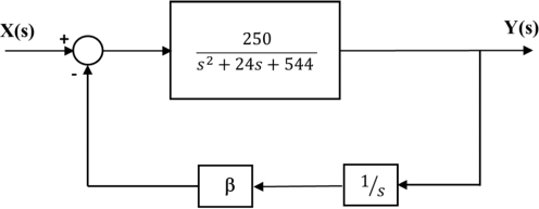
1.   Figure 1 shows the control block diagram of a dynamic model of the neuromuscular reflex, similar to but simpler than the model discussed in class. In this experiment on which the model is based on, the subject is seated comfortably, and his shoulder and elbow are held by adjustable supports so that the upper arm remains in a fixed horizontal position throughout the test. The subject’s forearm is allowed to move only in the vertical plane.

Before the start of the experiment, the angle between the subject’s forearm and upper arm is maintained and there is no angular motion (ie. angular velocity of the forearm is zero).

However, starting at time t = 0, an external torque x is applied to the arm. The external torque produces a change in angular velocity, y, of the forearm. In this version of the model, we assume that there are no delays in the closed-loop system.

The parameter β represents the overall gain for the entire feedback process: neural traffic from the muscle spindles to the spinal cord, the efferent neural drive from spinal cord to    biceps muscle and activation of the muscle to counteract the external disturbance.

a.   (15 pt) If β were to be effectively reduced to zero (eg. by pharmacologically blocking the transmission of afferent neural traffic from the muscle spindles to the spinal cord), determine an expression that shows how y would change with time in response to an impulsive change in external torque (ie. x(t) = δ(t)). Provide a rough sketch of the time-course in y(t).

b.   (15 pt) Suppose that, after reversing the neuromuscular blockade, we administer a drug that can enhance the neural traffic between the spindles and the spinal cord   and thus progressively increase β . Determine analytically (which stability analysis   method should we use?) the value of β at which y(t) begins to take the form of a     sustained oscillation in response to an impulsive disturbance in x(t).

Figure 1.

2.   Figure 2A shows a negative feedback system, and Figure 2B displays the Bode magnitude and phase plots of the frequency response of its loop transfer function, G(s)H(s). Note that the frequency axes in the graph are given in units of rad/s. From these plots, estimate the   following:

a.   (5 pt) Phase crossover frequency (in Hz) – mark this frequency with a circle “O” on Figure 2B;

b.   (5 pt) Gain crossover frequency (in Hz) – mark this frequency with an “X” on Figure 2B;

c.   (5 pt) Gain margin (in dB) – mark on Figure 2B with a circle “O” the point of magnitude plot at which you determined the gain margin;

d.   (5 pt) Phase margin (in degrees) – mark on Figure 2B with an “X” the point of the

phase plot at which you determined the phase margin;

e.   (5pt) Is this system stable or unstable? Briefly explain.

Figure 2A.

Figure 2B.