Hello, dear friend, you can consult us at any time if you have any questions, add WeChat: daixieit

Ordinary Differential Equations and Dynamical Systems

MATH 4400 – Fall 2021

Homework 1

        This homework has 100 points plus 25 bonus points available. Full credit will generally be awarded for a solution only if it is presented both correctly and efficiently using the techniques covered in the class and readings, and if the reasoning is properly explained. You will not generally receive full credit, even for a correct answer, if your method of calculation is less efficient than what you should be able to do based on the class. Substantial points on each problem will be associated with explicit statements concerning each concept you are using, and explanations for any numbers introduced in your calculations. You should simplify your expressions and answers as much as possible (either as a decimal or fraction), unless otherwise specified.

        Here are some recommended problems from the course text by Strogatz. They will not be graded, so you don’t need to write them up, but you should know or learn how to do them:

● 2.1.1, 2.1.2

● 2.2.1–2.2.10, 2.2.12

● 2.3.2, 2.3.3

● 2.4.1–2.4.8

● 2.5.2

● 2.6.1

        On the following pages are the problems assigned to be written up and submitted for grading.

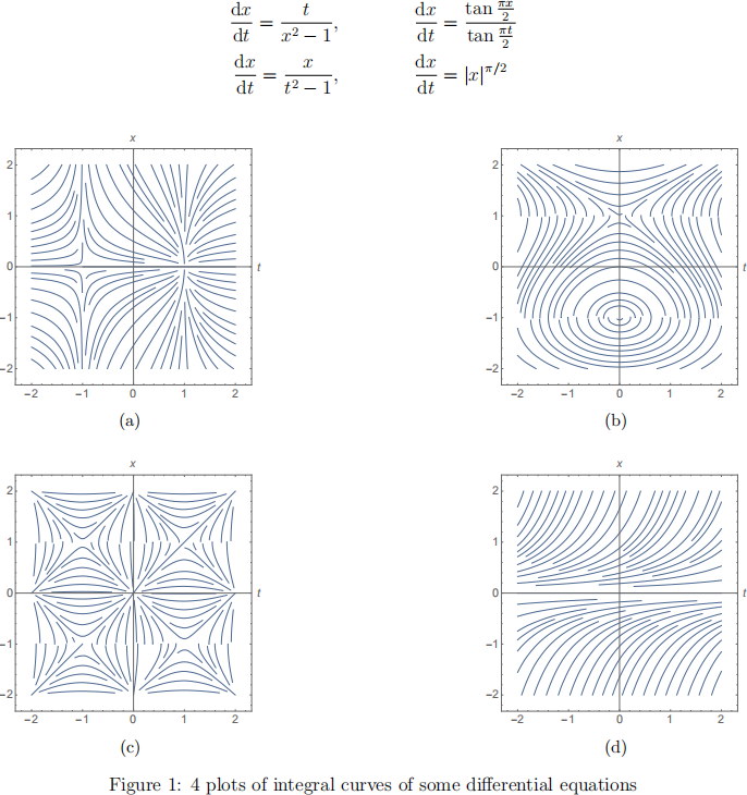
1 A matching problem (40 points)

Match each of the differential equations listed below to the plot indicating some integral curves of that differential equation. If you believe that no plot matches one or more of the differential equations listed, indicate this. Most of the credit is associated with an analytic explanation for your reasoning.

2 Another Kind of Symmetry for Differential Equa-tions (60 points plus 25 bonus points)

In class, we considered classes of differential equations of the form:

●  = f(t), for which vertical translations of integral curves give other integral curves, meaning that if x = (t) is a solution, then so is x = (t) + k for any real constant k

●  = f(x), for which horizontal translations of integral curves give other integral curves, meaning that if x = (t) is a solution, then so is x = (t + h) for any real constant h

Consider now a class of differential equations of the form

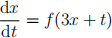
where f is an arbitrary smooth function.

a. (10 points) Find a group of transformations in the (t, x) plane that leave f(3x + t) invariant. As with the examples in class, look for a group of transformations describable by a single real parameter. Express the group of transformations in both analytical and geometric terms.

b. (10 points) Verify analytically (prove) that the differential equation (1) enjoys a symmetry under the group of transformations you found in part a, meaning that you can take any given solution (or integral curve) of the differential equation (1), apply the transformation from part a to it, and obtain another solution (or integral curve).

c. (10 points) Derive a general solution for the class of differential equations (1), which may be expressed implicitly in terms of the given smooth function f.

d. (5 points) Discuss technical limitations to the general solution you derived in part c.

e. (10 points) Plot the slope field and some integral curves for the differential equation

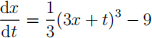
It is fine to provide either a hand-drawn or computer-generated plot, but substantial credit is associated with relating key features of the plot to the differential equation.

f. (5 points) Relate the symmetry property from part b for general smooth functions f to the direction field and integral curves you drew in part e.

g. (10 points) Suppose we find, by either analytical expression or numerical approxima-tion, a solution x = (t) to Eq. (2) satisfying the initial condition x(0) = 1. How could we obtain the solution to the differential equation (2) with different initial conditions x(0) = x0 from the solution in hand for x0 = 1 with a short computation that doesn’t require obtaining and manipulating the general solution nor a full recomputation from scratch? You do not need to obtain nor execute the short computation for the regular credit, but you are asked to provide a precise description of how you would process (t) to obtain the solution for x(0) = x0.

h. (10 bonus points) For what values of x0 should the short computation procedure from part g be expected work? Give a theoretical explanation for your answer. You do not need to implement the procedure to answer this question!

i. (15 bonus points) Execute the short computation procedure from part g. This of course requires you to obtain (t); I do not recommend computing this by hand. Rather I would suggest trying symbolic or numerical computation with your favorite mathematical software. Of course it would then be very easy just to change the initial condition and compute again, but pretend that solving the differential equation is too computationally expensive to repeat, and so once you obtain (t) you want to obtain the solution for different initial conditions by the short computation procedure you described in part g. Implement and illustrate this short computation for at least 3 different values x0 1. Plot the solutions you obtained in this way and show they are indeed integral curves of the slope field of Eq. (2).