Introduction

This practical covers buffering and overlay functions in ArcGIS Pro. The work also involves further work with attributes. The instructions in this practical will become less and less detailed as  you  are  now  expected  to  have  become  more  familiar  with  the  basic  functions  and operations of ArcGIS Pro.

Today’s practical

In  this  practical,  you’ll  conduct  a  simple  assessment  of  disturbance  to  ancient  woodland habitats in Cumbria. As part of the practical you will be identifying:

•    Sources of potential disturbance – for example road and rail corridors.

•    Relative patterns of exposure to disturbance – for this exercise we are assuming this is represented by proximity to built-up areas, road and rail transport.

•    Elements at risk and their vulnerability – in this exercise, parcels of ancient woodlands and their potential relative value as habitats.

Your analysis work will answer the question:  Which  ancient woodlands  in  Cumbria  are most at risk from disturbance?

NOTE:  Problems can and do occur due to  lack of space. You should allow  at  least 100MB for today’swork.

Table 1:  Input data to be used:

Table 2: Other data generated from the input datasets:

Getting the data

1.   Launch ArcGIS Pro

2.  When  prompted,  create  a  new  project  called  Practical3.  Save  this  directly  under  the existing  GEOG60951  directory.  ArcGIS  Pro  will  create  a  new  project,  folder  and geodatabase, all named “Practical3” .

3.   Download the data from  Blackboard  (Course Content  >  Block 2 > Week 3: Vector Overlay > Week 3 – Practical Materials > Week3.zip).

4.   Import the data over to your  Practical3.gdb geodatabase that ArcGIS Pro will have automatically created for you (right-click on your new geodatabase > import feature class(es)).

5.   Insert  a new map to your project and load all the layers from Practical3.gdb (Hint: search, select, and drag the layers into the map from Catalog pane).

Q1: What is the OS feature code for motorways in the Meridian dataset?

Q2. How many woodlands are contained in the ancient woodland dataset? What is their total area (in hectares) and the mean, min and max woodland sizes? (Remember you can right-click on any attribute field to select statistics).

Delineating a bounding polygon

This practical uses ancient woodland polygons for a defined county area. However, what if you didn’t have an appropriate boundary and wanted to define a study area for the polygons yourself? You can use a convex hull for this purpose – see below:

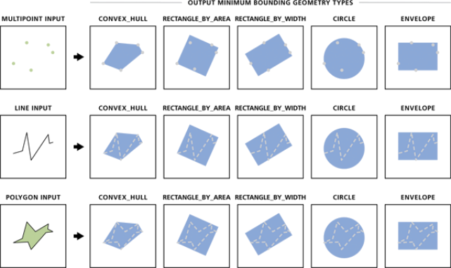
Types of minimum bounding geometries (Source: ESRI). Convex hull returns the smallest convex polygon that encloses a group of objects.

You can use the search function in ArcGIS Pro to find relevant tools:

1.  Go to Analysis  Tools. The Geoprocessing window opens.

2.  Type “convex hull” into the search window.

3.  Look for the  Minimum  Bounding  Geometry tool that you can  use to  carry out a convex hull operation (you may need to scroll down to find it). It shows you the location of  the tool (Data Management Tools), but you can also click on the link to open the tool directly from the search window.

4.  Open the Minimum Bounding Geometry tool and complete the tool window as follows:   Input features = ancient_wood; Output feature class = AW_boundary (saved  in your

Practical3 geodatabase); Geometry type = Convex hull; Group Option = ALL

5.  Run the tool and review the outputs.

Q3: What is the area of the convex hull describing the spatial extent of the ancient woodland layer?

Analysis Stage One - determining the severity / likelihood of disturbance hazard

The ‘A’ road and motorway buffers have already been generated before the practical. It just remains to carry out buffer analysis on the railway and urban area features.

(a) Creating buffers around railway features

1.   In the Geoprocessing pane, click on Toolboxes to reveal the

list of available Toolboxes. Within this list, go to Analysis

Tools > Proximity > Multiple Ring Buffer and click to operate

the tool.

2.   For  Input  Features select the railways layer. Call the new

file buffRail and save to your Practical3.gdb

3.   In the distance box type 500, then click “Add another” and

then type 1000 in the second box. Note, these refer to 500

metres and 1000 metres (rather than feet, yards, miles, or

some other distance measurement). This is defined by the

coordinate  reference  system  that  is  being  used.  As  this

practical  uses  data  for  the  UK,  we  are  using  the British

National Grid, which uses metres as its linear unit.

4.   Click Run. When processing is complete the railway buffer layer is added to the map automatically.

5.   Save your project before moving on.

(b) Updating the attribute table of the new buffRail data layer.

You now need to modify the attribute table so that we have a set of codes relating the severity and/or likelihood of disturbance hazard to each of the buffer zones. To do this we will add a field called Rail_code to the attribute table and update the values by hand.

1.   Right click the layer name (buffRail) and select Attribute Table

2.   Click Add Field. Call the field Rail_code and change the data type to Short (Integer). For the number format, choose Numeric and leave the default options (i.e. rounding, alignment). Click Save on the “Fields” tab > Changes panel which should have appeared on the main ribbon.

Save “Add field”

You should see a field called Rail_code added to the buffRail attribute table.

3.   Move your cursor over the rows in the Rail_code field and double-click on one of the rows.

4.   Type  in  new  values  for  the  Rail_code  field.  For  rows  with  a  value  of  500  in  the distance field type 2 and press <Enter> and for rows with a value of 1000 type 1 and press <Enter>. This is to signify a higher exposure to the hazard (i.e. closer to the source of the disturbance).

5.  View your results by right clicking on buffRail in the contents pane and going to the symbology tab.

6.   Change the colours for each Rail_code value (> Unique Values and choose RailCode from the field menu).

7.   Save your edits and the project.

(c) Creating buffers around urban area features

You are now going to create another multi-ring buffer, selecting the urban feature class layer as the features to buffer. Opt to create a multiple ring buffer, one at 500m and the other at 1000m (call it buffUrban).

Q4: Explain the polygon buffer process (i.e. how is the buffer created).

Q5: Why might you want to buffer inside a polygon rather than outside it? Suggest one application for inside polygon buffer analysis.

(d) Updating the attribute table of the new buffUrban data layer.

As with the buffRail feature class layer, you now need to modify the attribute table so that we have a set of codes relating the degree of hazard exposure to each of the buffer zones. To do this, we will add a field to the attribute table and update the values using a database attribute query  and  the  calculate  command.  This  is  an  alternative  means  of  changing  /  modifying attribute values if there are too many to update them all by hand as in the previous example.

1.   Right click the layer name (buffUrban) and select Attribute Table.

2.   Click Add Field. Call the field Urban_code and set the field type as a Short Integer and the Number format as Numeric. Click Save on the Field tab.

3.   Close the “Fields: buffUrban” tab. Now, from the Map tab on the main ribbon, navigate to Selection > Select By Attributes.

4.   For the input rows, select buffUrban and keep the Selection type as “ New selection”

5.   Click + New Expression (if not visible) and try to work out the selection query needed to select records associated with the 0m–500m buffer (high disturbance).

6.  When you think you’ve got it, press Apply and the buffUrban layer should now have highlighted all the cases that meet the selection criteria.

7.   Right click the Urban_code title (with the Attributes Table) and go to Calculate Field. In the field calculator screen, add the value of 2 underneath the label ‘ Urban_code =’ . Click Apply and this will update the values for this selection to 2, representing the nearest buffer zones. Make sure to clear the selections.

8.  Adapt steps 4 – 7  to give a value of 1 to the buffer zones furthest away from the urban features.

9.   In the Selection panel of the main toolbar click Clear.

10. View your results by right clicking on the buffUrban layer and selecting Symbology as before. Be sure to check the results appear logical and expected.

The other buffer zones (Motorways, A roads) have already been created for you, along with their respective disturbance codes (Mway_code, Aroad_code). You’ll need these later. You’ve now done a lot of work, save your project.

(e) Overlaying buffer zones.

All of the buffer zones, except for the buffRail have already been overlaid to combine them. You can have a look at the results in the data layer called allexceptrail in the Practical3 geodatabase. Add this layer to your project now if you haven’t done so already. This only needs the railway buffers adding before the combined disturbance code taking account of the motorways, A roads, railways and urban areas can be calculated. Take a look at the attribute table of the allexceptrail layer to see the fields that this layer already contains. We’ll now add the final disturbance factor to this layer.

Q6: Explain the difference between union and intersect overlay operations. How does the intersect operation here differ from the one carried out in the select by location window (i.e. as used in the Formative practical, Practical 1)?

1.  With the Analysis tab selected from the main ribbon, open the Union tool from the Tools Gallery, or find it within Tools > Toolboxes > Analysis Tools > Overlay.

2.   From  the  Geoprocessing  pane  –select  the  buffRail  layer  as  the  first  input  layer  to overlay.

3.   Next select the allexceptrail layer as the second input layer.

4.   Leaving  all  other settings  as the default,  in the  output feature class  box,  go to your Practical3 geodatabase and save the output layer as allbuffers. Keep the option to join all attributes.

5.   Click Run and wait. When processing is complete, the new layer is automatically added to the Contents pane.

6.   Click on the new allbuffers layer, right click and go to Attribute Table. You should be able to see that Rail_code is now one of the attributes associated with this layer. You should also be able to see Urban_code, Aroad_code and Mway_code which indicate the levels of potential disturbance associated with each. There will also be some other fields that you no longer need. We’ll first delete them before adding some new fields that we’ll need later on in the analysis.

7.   Go to Fields and then Add Field, name the field Tot_code, keeping the defaults for the field attributes. Tot_code should now appear in the attribute table. Repeat this process to add a field called Fin_code. Click save from the Fields tab.

8.   From  the  allbuffers  attribute  table  we’ll  calculate  some  values  for  Tot_code  and Fin_code. First click on the column heading for the Tot_code field, right click and click Calculate Field. A new window appears. You’ll notice that the [Tot_code] = is already specified, you only have to give the value or calculation needed in the box underneath.

9.   The  next  stage  is  to  specify  the  calculation.  We  want  to  add  up  the  codes  from Rail_code,  Urban_code,  Mway_code,  Aroad_code  and  put  the  results  into  the Tot_code field. To do this double-click on Rail_code in the Field list, click +, double-click on  Urban_code,  click  +,  double-click  on  Mway_code,  click  +  and  double-click  on Aroad_code.  You  should  see  your  calculation   being  added   (e.g.   !Rail_code!   + !Urban_code! +  …  ).  Check that this is correct by clicking the green tick button (you should get a message back ‘Expression is valid’). Once your expression is confirmed as valid click Apply and the Tot_code field should update with the results of the calculation.

10. Now  we  want  to  update  the  values  in  the  Fin_code  field.  In  practical  1  you  did  a calculation function when calculating population density for all fields (or all polygons) in the data layer. This time we want to do a calculation on selected subsets of the fields (or polygons) in the data layer that conform to different criteria and then allocate different values to each. The basis of the differences are as follows:

. Very severe disturbance (Fin_code = 4 for buffer areas with a Tot_code value >=6

. Severe disturbance (Fin_code = 3 for buffer areas with a Tot_code value >=4 to <6

. Medium disturbance (Fin_code = 2 for buffer areas with a Tot_code value >=2 to <4

. Low disturbance (Fin_code = 1 for buffer areas with a Tot_code value <2

11.  To achieve this, we will use a series of “if” statements in Python 3 code.

12.  First right-click on the Fin_code field and select Calculate Field.

13.  In the box beneath “Fin_code=” type: Total(!Tot_code!)

14.  In the “Code Block” box type or paste the following code:

def Total(value):

if(value >= 6):

return 4

if(value <6 and value >=4): return 3

if(value <4 and value >=2 ): return 2

if(value <2):

return 1

15. Select the green tick button to check the expression is valid. If it is not valid, it is likely

due to indentation of the final line (return 1).

16. Once valid, click “Apply” .

17. You can now view the results of your work. Click on the allbuffers layer, right click on Symbology. Click Categories and Unique Values. Select Fin_Code from the value field drop down box. You should have four categories, if not, select More (above the classes table) and choose ‘show all other values’ . If you prefer you can alter the labels and the colours to make your data layer easier to understand and to view. Try removing the outline to make the features easier to see (Left click on the colour symbols in turn to make these adjustments or Format all symbols under the More drop-down menu). Ask if you are not sure.

At this point, you can clear up some of the files you no longer need and free up some disk space. You can now delete the allexceptrail, buffRail and buffUrban data layers from your geodatabase  and   Practical3  directory   and  compact  the  database  to   minimise  space requirements.

1.   First remove the layers specified above from your contents pane.

2.   Save your project.

3.   Open the CatalogView pane.

4.   Delete the allexceptrail, and buffUrban layers from the Practical3 geodatabase then compact the database by right clicking on it > Manage > tick Compact > click OK. If it doesn’t compact for some reason, and you’ve plenty of space, just continue for now.

Analysis  Stage  Two  -  determining  the  degree  of  vulnerability  associated  with  the woodlands

The next set of criteria estimate the degree of loss or damage associated with different parcels of ancient woodland. You’ll remember that we are assuming that the most valuable tracts of ancient woodland are those which are:

•    Made up of semi-natural (as opposed to replanted) growth - this will be generated by carrying out an attribute query to classify woods as high ecological value. You will put the results in a field called Vuln_code which has already been created for you.

•    Within the national park - this will be generated by firstly using a spatial query to select all parcels within the national park polygon and secondly adding an attribute field to mark these woodlands  as  high  protection  value.  You  will  be  adding  an  additional weighting to the Vuln_code field for the polygons which are within the national park (Lake_District  layer).  Overall  vulnerability  will   be  estimated  using  the   following hypothetical guidelines:

. High vulnerability – woodlands with both high protection and high ecological value

. Med vulnerability – woodlands with either high protection or high ecological value

. Low vulnerability – woodlands with neither high protection or high ecological value

1.   Open  the  Attribute  Table  for  the  ancient_wood  data  layer.  On  the  main  toolbar navigate  to,  Map  >  Select  By  Attributes.  Add  Clause  WOOD_TYPE  is  Equal  to Replanted and then and Apply to select records satisfying that search criteria.

2.   Now right click the Vuln_code field label in the Attributes Table and select Calculate Field. Add a value of 1 to the blank box so that the calculation reads Vuln_code = 1. Click Apply and OK to populate the Vuln_code field with the value of 1 for all the selected records.

3.   Now go to click Switch Selection at the top of the Attribute Table to select all the other records in the database. We can do this because there are only two categories in the Wood_type field: “replanted” and “semi-natural” . We now want to select everything which is not “replanted” – i.e. that is “semi-natural” .