闪电代写 -代写CS作业_CS代写_Finance代写_Economic代写_Statistics代写_代码代做_IT代写_加急帮助

Hello, dear friend, you can consult us at any time if you have any questions, add WeChat: daixieit

Coursework: Search for a magnetic skyrmion

Computational science is emerging as the third pillar of research and development in academia and industry across all science and engineering disciplines. Computational studies complement experimental and theo- retical approaches and are sometimes the only feasible way to address research challenges, effective indus- trial design, and engineering of various products and systems. For example, in nanomagnetism – a ﬁeld of physics predicting the magnetic behaviour of systems at nanometer scales – simulations have become well- established. They are often the only possible technique for exploring different magnetic phenomena of funda- mental physical interest and their applications in data storage [1, 2],information processing [3, 4], medicine [5], and many other ﬁelds. Their use becomes more widespread and reliable as the models, simulation techniques, and computational power advance. In research, we use computational magnetism to verify theory, explain and guide experiments, and propose designs for different spintronic nano-devices.

Different models with different levels of abstraction and complexity are used in computational magnetism. Each model has its advantages and disadvantages. In this coursework, we will implement a Python-based Metropolis Monte Carlo simulator using the Heisenberg spin model on a two-dimensional spin-lattice and employ it to ﬁnd a magnetic skyrmion [6, 7]. Magnetic skyrmions – topologically stable quasi-particles – have become a topic of intensive research due to their promising properties to revolutionise how we store and process data [8 – 10].

It could be much work, so let us slowly introduce different concepts and give guidance on how to reach the solution.

Atomic spin and spin lattice

As children, we played with magnets and experienced attractive or repelling forces between them. Later in school, we learned that magnet is a dipole – it has its north (N) and south (S) pole as we show in Fig. 1 (a). If we attempt to cut a magnet into smaller pieces, as we show in Fig. 1 (b), each piece will again be a dipole with both N and S poles. More precisely, we cannot (or still do not know how to) isolate a magnetic monopole.

For simplicity, instead of drawing a magnet as a rectangle with marked north (N) and south (S) poles, as a convention, we draw a single vector as we show in Fig. 1 (c). We call that vector the magnetisation vector M1 . Its head (tip of the arrow) corresponds to the north pole, whereas its tail corresponds to the south pole.

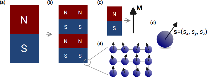
Figure 1: The concepts of magnetic poles, magnetisation vector, lattice, and spin. (a) Each magnet has its north (N) and south (S) poles. By cutting the magnet into smaller pieces as shown in (b), we cannot isolate a magnetic monopole – each piece is again a magnetic dipole with both poles. For simplicity, instead of drawing a picture of a magnet with N and S poles, we draw a magnetisation vector M with its head and tail corresponding to the north and south poles, respectively. (d) If we keep zooming in, we will see that the smallest magnets are atoms arranged in a lattice. (e) The basic building block of the Heisenberg model is a spin vector s.

We already said that cutting a magnet into smaller pieces results in magnetic dipoles. Now, think about the smallest magnetic dipole we can cut out. As we show in Fig. 1 (d), if we zoom in sufﬁciently, we can notice that magnetic materials (or at least the ones we are exploring in this coursework) consist of atoms in symmetrical structural arrangement. We call such a symmetrical structural arrangement a crystal lattice. Therefore, this implies that the smallest magnetic dipole is associated with an individual atom in a crystal lattice, as shown in Fig. 1 (e), and we can understand the behaviour of a magnet as the collective behaviour of individual atomic dipoles. Accordingly, the basic building block in our simulations will be an atomic dipole. In literature, people use different names for atomic dipoles, for instance, magnetic moments, atomic moments, or spins. This work will refer to them as spins s.

Many concepts in magnetism have their roots in quantum physics. We do not have time or ambition to dive into the quantum world as part of this coursework since we have to begin developing our simulator. Therefore, we will use the (simpliﬁed and modiﬁed for this work) Heisenberg’s spin model and summarise it with the following approximations:

. Atoms are arranged in a two-dimensional (2D) lattice as shown in Fig. 2.

. Atoms have a ﬁxed position in space, i.e. their distance from the nearest neighbours (lattice constant a) is constant in space and time.

. All atoms are magnetic: each atom has a spin s, which is a vector s = (sx ,sy , sz ) that can point in any

direction in a three-dimensional space.

. The magnitude of all spins is constant: |s| = 1.

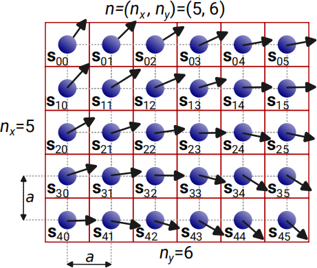
Figure 2: An example of a two-dimensional lattice of classical Heisenberg spins. Atoms are arranged in a two-dimensional crystal lattice with lattice constant a. Each atom in the lattice is magnetic and has the spin s, which is a vector that can point in any direction in the three-dimensional space s = (sx ,sy , sz ). The norm (magnitude) of all spins is constant in both space and time and equals to 1.

One of the main tasks of computational magnetism is to explore the collective behaviour of spins, i.e. to ﬁnd out in what direction each spin in the lattice is pointing. In Fig. 2, we show an example lattice with nx = 5 and ny = 6 atoms in the x andy directions, respectively. Each atom has its spin si,j . The upper left spin, we mark with s0 ,0, whereas the lower right spin is s(nx −1,ny − 1) = s45 .

We will model and implement the spin-lattice in our simulation code using Spins class. In mcsim/spins.py, you can ﬁnd the skeleton of the Spins class with init and some other methods already implemented. We can see that the data structure holding values of all individual spins array is a NumPy array. Its shape is (nx , ny , 3), where nx and ny are the number of spins in x andy directions, respectively, and 3 because each spin has three components (sx ,sy , sz ). For instance, to access the y-component of the second spin from the top and the third from the left, we would write array[1,2,1]. Before introducing further concepts, let us begin coding and introduce several tasks.

Task 1: mean property

Instead of looking at the values of individual components of all spins in array to inspect what magnetisation state has emerged in our lattice at the end of the simulation, we often use aggregates. One of them is the mean. In this task, implement the mean property in Spins class. It returns a NumPy array2 [¯(m)x , ¯(m)y , ¯(m)z ], where ¯(m)c for any component c = x,y,z is computed as

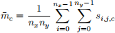(1)

Tests that could guide you to the solution are in tests/test spins.py::TestMean .

How do I run tests? In this work, we are using pytest package to test our code. All tests can be found in mcsim/tests/test *.py ﬁles, and if you do not have Pytest installed, you can install it in your conda environ - ment using pip install pytest.

We run pytest by typing pytest in our repository, or if we want a more detailed output, we run pytest -v. Pytest will then explore all ﬁles in our repository and its subdirectories to ﬁnd the ones whose ﬁlename begins with test and execute all functions/classes that begin with test or Test.

In each test, we perform a particular set of commands and check their output using an assert statement. Suppose the expressions in all assert statements result in True; our test passes. Otherwise, it fails, and from the output Pytest gives us, we can see why, i.e. we can compare the output we got with the expected output. Please note that even if your tests fail, it does not mean you will get zero marks for your implementation. We will examine all functions carefully. On the other hand, if the tests are passing, it does not mean you will get the maximum points for that task. You do not have to run the tests - they are not mandatory. They are simply there to help you with your code development, but you do not have to run them. If you believe they are a distraction, please ignore them.

All tests will fail the ﬁrst time you clone your repository and run pytest. This is because some methods rely on others. So, for tests to pass for one method, other methods need to be implemented. As you progress implementing your code, more tests will be passing. Running Pytest requires your code to be packaged, or at least init .py ﬁles to be present in your repository. Because of that, we have already given you those ﬁles so that you can run tests from Task 1.

Task 2: abs special (dunder) method

When we introduced the concept of the simpliﬁed and modiﬁed Heisenberg model of spin-lattice, one of the approximations was that the magnitude of spins, i.e. the norm, is constant, does not vary in space and time, and it equals 1. Therefore, one of the operations our Spins class should do is to compute the norm of all spins in the lattice. Instead of naming the method, for instance, norm or magnitude, we will overload abs operator so that when we call the built-in abs function on an object, which is an instance of Spins class, that method will be called to calculate the norm (magnitude) of all spins in the lattice. In this task, implement abs special (dunder) method, which returns a NumPy array with shape (nx , ny , 1). The norm of a spin at location i,j is computed as:

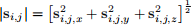(2)

To know whether your function is returning expected solutions for some of the tested cases, please refer to the tests in tests/test spins.py::TestNormalise .

A good start! We have introduced the concepts of spin and spin-lattice, gave an overview of approximations we will use, and even began coding by attempting to implement two methods to extend the capabilities of the Spins class. Let us explore how spins interact with each other and the environment by introducing four energy terms we will use to compute the system’s energy (Hamiltonian).

Zeeman energy

The ﬁrst energy term we will introduce is the Zeeman energy term. We know that if a magnetic dipole (e.g. a magnetic needle in a compass) is placed into an external magnetic ﬁeld (e.g. Earth’s magnetic ﬁeld), it will tend to align itself parallel to the external magnetic ﬁeld. The energy responsible for this is the Zeeman energy.

If we have an spins, placed into an external magnetic ﬁeld B, as we show in Fig. 3 (left) we can compute the Zeeman energy as

(3)

Let us now consider how this expression means that the spins wants to align itself with the external mag- netic ﬁeld B. All physical systems tend to reduce their energy and be in the state of (local) minimum energy.

If we say that the angle between s and B is θ, then the Zeeman energy would be ez = −|S||B|cosθ . For what angle θ does the Zeeman energy have the minimal value? Due to the minus sign in front, it will be for θ for which cosθ has the maximum value 1. Accordingly, for θ = 0, Zeeman energy is at its minimum, which is why it tends to align the spin parallel (in the same direction) as the external magnetic ﬁeld as we show in Fig. 3 (right).

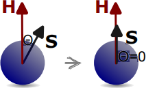
Figure 3: Zeeman energy. The Zeeman energy of an individual spin s in an external magnetic ﬁeld B is ez = −s · B. Therefore, Zeeman energy tends to align the spin parallel to the external magnetic ﬁeld.

We compute the Zeeman energy for the entire two-dimensional lattice as the sum of energies for all spins.

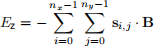(4)

Task 3: zeeman method

The arrangement of spins, together with all the parameters we need to compute the total energy of the system will be provided by the user when they deﬁne an object of System class. You can ﬁnd the System class in mcsim/system.py. In this task, implement zeeman method of the System class. This method should return the total Zeeman energy of the system as a float computed using Eq. 4. If we have a look at the init method of the System class, we can see that the attributes we need to implement zeeman method are self.B and self.s.array.

The relevant tests for this implementation can be found in tests/test system.py::TestZeeman .

Uniaxial anisotropy energy

When atoms are arranged in a lattice, most often, unless the material is isotropic, certain directions are prefer- ential for the spins to be aligned to. The energy “responsible” for that alignment is called the anisotropy energy. Different types of anisotropy exist, each with a different expression for computing the total energy. However, in this work, we will implement the uniaxial anisotropy energy. It tends to align spins s parallel or anti-parallel to

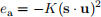(5)

where K is the anisotropy constant, which depends on the material we are simulating, and u is the anisotropy axis. Often, we assume that the anisotropy axis is a unit vector (its magnitude is 1): |u| = 1. We can compare Eq. 3 and Eq. 5 and notice the difference in the square of the dot product. Accordingly, unlike Zeeman energy, which tends to align all spins parallel to the external magnetic ﬁeld, uniaxial anisotropy energy wants spins aligned parallel or anti-parallel to u.

The total uniaxial anisotropy energy of the entire system is

nx −1ny −1

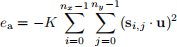(6)

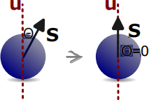
Figure 4: Uniaxial anisotropy energy. The uniaxial anisotropy energy of an individual spins with anisotropy axis u and the anisotropy constant K is ea = −K(s · u)2. Accordingly, uniaxial anisotropy energy tends to align the spin parallel or anti-parallel to the anisotropy axis u.

Task 4: anisotropy method

Implement anisotropy method of the System class. This method should return the total anisotropy energy of the system as a float computed using Eq. 6. Uniaxial anisotropy parameters K and u will be provided by the user when they deﬁne the System object. However, as we mentioned previously, we assume that the norm (magnitude) of u is normalised to 1 before computing the energy (|u| = 1). Therefore, inside the anisotropy method, ensure that u is normalised before computing the energy. If we have a look at the init method of the System class, we can see that the attributes we need to implement anisotropy method are self.K, self.u, and self.s.array.

The relevant tests for this implementation can be found in tests/test system.py::TestAnisotropy .

Exchange energy

So far, we explored the Zeeman and uniaxial anisotropy energy terms. Those energies are “local” – spins tend to align to an external magnetic ﬁeld or the anisotropy axis, independent of the neighbouring spins in the lattice. In this work, we will implement and use two energy terms we call short-range interactions – to ﬁnd the spin’s preferential direction, we must consider the spins of the nearest neighbours.

The ﬁrst short-range energy term is the exchange. If we have two neighbouring spins s1 and s2 (isolated or in a lattice), the exchange energy between them is

(7)

where J > 0 is the exchange energy constant, depending on the material we are simulating. From this expres- sion, we can see that, since J > 0, exchange energy between spins s1 and s2 will be at its minimum when they are parallel to each other – they are pointing in the same direction, as we show in Fig. 5. Exchange energy does not introduce any preferential direction like Zeeman and anisotropy energies. It only tends to align all spins parallel to each other.

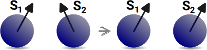
Figure 5: Exchange energy. The exchange energy between two spins s1 and s1 is eex = −Js1 · s2, where J > 0 is the exchange energy constant. Therefore, exchange energy tends to align neighbouring spins parallel to each other and does not have a preferential direction.

We already mentioned that the exchange energy is a short-range energy -each spin tends to be parallel to its nearest neighbours. To clarify, if we look at the lattice of spins we showed in Fig. 2, as an example, the nearest neighbours of the spins1 , 1 are s0 , 1, s1 ,0, s1 ,2, and s2 , 1. Spins across the diagonal of the unit cell, e.g. s0 ,2, are not the nearest neighbours. Therefore, we compute the total exchange energy as the sum of exchange energies between all nearest neighbours.

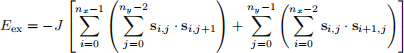(8)

Task 5: exchange method

Implement exchange method of the System class. This method should return the total exchange energy of the system as a float computed using Eq. 8. A user provides an exchange energy parameter J > 0 when they deﬁne the System object. The attributes of the System class we need to implement exchange method are self.J and self.s.array.

The relevant tests for this implementation can be found in tests/test system.py::TestExchange .

Dzyaloshinskii-Moriya (DMI) energy

Although this energy term has been well understood for over 50 years, it became the focus of intensive research only after it was predicted that it could give rise to non-trivial magnetisation states in nanomagnetic systems, such as magnetic skyrmions. Like the exchange energy, this term is short-range, and the direction a spin wants to align depends on the nearest neighbouring spins.

If we have two neighbouring spins s1 and s2, the Dzyaloshinskii-Moriya (DMI) energy between them will be

(9)

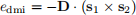
where D is the Dzyaloshinskii-Moriya vector, and it depends on the material we are simulating. In contrast with the exchange energy we introduced previously, the material parameter D is a vector. From the energy expression for the two spins, we can see that this energy is minimal when spins s1 and s2 are perpendicular to each other (due to the cross product) and in the plane that is perpendicular to D, as we show in Fig. 6. Therefore, DMI energy tends to align spins perpendicular to its neighbours.

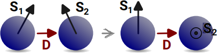
Figure 6: Dzyaloshinskii-Moriya (DMI) energy. The DMI energy between two spins s1 and s1 is edmi = −D · (s1 × s2 ), where D = Drij is the DMI vector. DMI vector in this work is a vector with magnitude D (DMI parameter) and in the direction from s1 to s2 . DMI energy tends to align neighbouring spins perpendicular, in the plane which is perpendicular to vector D.

The Dzyaloshinskii-Moriya energy term occurs due to the magnetic systems’ lack of inversion symmetry. This is either due to the non-centrosymmetric crystal lattice or because we have introduced asymmetry by stacking layers of different materials. In this work, we will consider the DM vector to be the consequence of the non-centrosymmetric crystal lattice, and in that case, the DMI vector between two nearest neighbouring spins s1 and s2 is

D12 = Dr12 (10)

where D > 0 is the DMI constant andr12 is a unit vector (|r12 | = 1) pointing from s1 to s2 . Accordingly, the total DMI energy for the entire two-dimensional lattice is

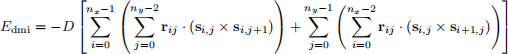(11)

Task 6: dmi method

Implement dmi method of the System class. This method should return the total Dzyaloshinskii-Moriya energy of the system as a float computed using Eq. 11. DMI energy parameter D > 0 is provided by a user when they deﬁne the System object. The attributes we need to implement dmi method are self.D and self.s.array. Please note that self.D is a scalar and not a vector. Therefore, the vector rij should be implemented implicitly in the calculation of the DMI energy.

The relevant tests for this implementation can be found in tests/test system.py::TestDMI .

Metropolis Monte Carlo algorithm

We have now introduced and implemented all energy terms we need to obtain a magnetic skyrmion emerging in a two-dimensional spin-lattice. So, for any spin conﬁguration, we can compute the system’s total energy as the sum of all individual energy terms by calling the energy method of the System class. We will introduce the Metropolis Monte Carlo algorithm to minimise the system’s energy and ﬁnd the conﬁguration of spins for which the energy is at a minimum. We call such conﬁgurations (or states) equilibrium states. For simplicity, we will assume we are minimising the energy of our system at zero temperature (T = 0).

The Metropolis Monte Carlo algorithm is performed by executing the following steps:

1. Compute the total energy of the system E0 .

2. Randomly select one spin in the lattice. Randomly selected spinsi,j must be drawn from a uniform dis- tribution, i.e. each spin must have the same chance to be selected.

3. Randomly change the spin’s direction to si(′),j . To perform this step, use function random spin(s0, alpha=0.1)

in mcsim/driver.py, where s0 is the original spin you are changing.

4. Compute the total energy E1 of the system with modiﬁed spinsi(′),j .

5. If the energy of the system after a random modiﬁcation of a spin has dropped (ΔE = E1 −E0 < 0), accept the changed spin and go back to step 1. On the other hand, if the total energy of the system has increased (ΔE = E1 − E0 ≥ 0), reject the changed spin. In other words, return the original value of the spin and go back to step 1.

We repeat those steps n times. Usually, depending on the size of the system we are simulating,n varies. In this work, we will use the values of n on the order of 105 − 106 .

Task 7: drive method

Implement the drive method of the Driver class. This method accepts an object which is an instance of System as an input parameter and the number of iterations n. It does not return anything, but it modiﬁes the system object passed to it. To access spins of the system, you need to access system.s.array. Similarly, to compute the system’s energy, you will be calling system.energy().

The relevant tests for this implementation can be found in tests/test driver.py .

Visualisation

We have now implemented all the necessary functionality to compute and minimise the energy of a two- dimensional spin-lattice to run a simulation. We will now implement the plot method in the Spins class, which we will use to visualise the spin lattice.

Task 8: plot method

You may have noticed that we missed implementing the plot method in Spins class. We will do it now since this is the main objective of this task. You have the freedom to design and implement the plot method to visualise the lattice of spins so that

. It is called by running system.s.plot() inside Jupyter notebook.

. You can add as many keyword arguments to the plot method. However, we should be able to call the plot method without passing any parameters. Therefore, please ensure the default values of keyword arguments are the ones you would like to see your plots with.

. You can only use matplotlib as a plotting package when implementing your function.

There are no tests associated with this method. However, please ensure your implementation of the plot method works by running and saving the notebook in my-research/magnetic-skyrmion.ipynb. The result of your visualisation should be saved as the output of the last cell in that notebook.

Optimisation

While you were working on the tasks, you might have already used some of the optimisation techniques. In the Metropolis Monte Carlo algorithm we implemented, each iteration should be performed as fast as possible because we usually run the algorithm in many iterations. Therefore, how can we optimise our code?

Task 9: Optimisation

In this task, optimise the code you have written and make the necessary changes to improve its perfor- mance. You are not required to modify any of the code we gave you.

Documentation

Task 10: Documentation

We have already discussed the importance of documentation, so let us introduce a task in which we can document our code. In this task, document your code and project.

Packaging

Let us ensure our simulation code is packaged for use in our research and for others who want to perform Metropolis Monte Carlo simulations.

Task 11: Packaging

In this task, package your simulation code. Please pay attention to the following points

. The package name is mcsim.

. Modify init .py ﬁles if necessary inside mcsim directory and its subdirectories.

. All dependencies – libraries required to run mcsim package – must be speciﬁed in requirements.txt ﬁle.

. Write setup.py ﬁle so that mcsim package can be installed by running

pip install .

. Apart from the package name, please feel free to choose the values for other parameters of the setup function in setup.py.

We will install and run your code in a well-deﬁned way, so please ensure your code is packaged and struc- tured so that the following steps can be executed:

1. We create a clean conda environment with Python 3.11 (conda create -n mcsim python=3.11) and ac- tivate it (conda activate mcsim).

2. We clone your repository by running git clone url to your github repository

3. We install mcsim package – ﬁrst we navigate into your repository (cd your-repository-name) and then

“pip-install” it (pip install .). Please note that we will run the pip install . command in the directory where mcsim directory and setup.py are.

4. We run tests with pytest in the same directory.

5. Finally, we will re-run your notebook.

Magnetic skyrmion

We have now implemented everything we need to run a simulation and attempt to ﬁnd a magnetic skyrmion.

Task 12: Magnetic skyrmion

In my-research/magentic-skyrmion.ipynbJupyter notebook, you will ﬁnd the simulation workﬂow. In this task, run all cells in the simulation workﬂow notebook and save it.

Please note that although the main objective of this coursework was to ﬁnd a magnetic skyrmion, running my-research/magentic-skyrmion.ipynbJupyter notebook might not result in one even if you implemented all methods correctly. Metropolis Monte Carlo simulation algorithm includes randomness, and we might end up in a local minimum equilibrium state in the energy landscape that does not correspond to a magnetic skyrmion.

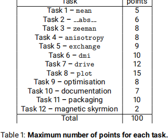
Points

The maximum number of points that can be given for each task is given in Table 1.

Comments

. The submission deadline is Friday, 20th October 2023, 16:00 BST. Please ensure everything is committed and pushed to your assessment repository before the deadline.

. We will run Q&A sessions on Wednesday 18th and Thursday 19th October at 16:00 BST. Wednesday’s session will be recorded, and in-person attendance is not required.

. All questions you may have related to this assessment must be posted to the Assessment 2 channel so that all students can see the answers and potentially beneﬁt from them.

. You cannot change any class’s signature or function, except for the plot function in Spins class. However, you cannot change the name of any method or class.

. You are free to introduce additional functions or classes if they help with the implementation of tasks.

. Nothing is perfect. Although we invested considerable effort to ensure this assessment document does not contain typos or mistakes, some might still be there. If you believe you spotted one, please let us know on the Assessment 2 channel as soon as possible, and we will clarify it for you.

. In this coursework, you are allowed to use ChatGPT. However, you must declare its use in references.md and explain how you used it.

Plagiarism

. Plagiarism is presenting work created by someone else or generated by an AI tool as your own. It is taken very seriously and dealt with according to the Academic Misconduct Policy and Procedure.

. Although using AI tools, e.g. ChatGPT or GitHub Copilot, is permitted, you must clearly acknowledge if and how you used them in your submissions. For further details, please refer to Conversational AI Tools Guidance3 .

. Although students are encouraged to discuss the problem background and coding techniques with their peers, you should not allow other students to examine your code, nor attempt to view the code of others. In cases of doubt, students may be examined on their submission via oral assessment.

. Add ALL references (articles, webpages, books, etc.) you consulted and used to references.md. For each reference, clearly explain what idea or code you have taken. In addition, cite appropriately in your code using comments whenever necessary. In the same ﬁle, explain how you used AI tools, if any.

References

1. Wood, R., Williams, M., Kavcic,A. & Miles,J. The Feasibility of Magnetic Recording at 10 Terabits Per Square Inch on Conventional Media. IEEE Transactions on Magnetics 45, 917–923 (2009).

2. Parkin, S. & Yang, S.-H. Memory on the racetrack. Nature Nanotechnology 10, 195–198. https://doi.org /10.1038/nnano.2015.41 (Mar. 2015).

3. Raab, K. et al. Brownian reservoir computing realized using geometrically conﬁned skyrmion dynamics. Nature Communications 13. https://doi.org/10.1038/s41467-022-34309-2 (Nov. 2022).

4. Zhang, X., Ezawa, M. & Zhou, Y. Magnetic skyrmion logic gates: conversion, duplication and merging of skyrmions. Scientiﬁc Reports 5. https://doi.org/10.1038/srep09400 (Mar. 2015).

5. Li, W., Liu, Y., Qian, Z. & Yang, Y. Evaluation of Tumor Treatment of Magnetic Nanoparticles Driven by Ex- tremely Low Frequency Magnetic Field. Scientiﬁc Reports 7. https://doi.org/10.1038/srep46287 (Apr. 2017).

6. Rßler, U. K., Bogdanov, A. N. & Pﬂeiderer, C. Spontaneous skyrmion ground states in magnetic metals. Nature 442, 797–801. https://doi.org/10.1038/nature05056 (Aug. 2006).