STA305H1F Section L0101 Homework: HW2
Hello, dear friend, you can consult us at any time if you have any questions, add WeChat: daixieit
Department of Statistical Sciences
Courses: STA305H1F Section L0101
Homework: HW2
Due date: 20 October 2023
0. Read the Assignment descriptions, information inside each box for submitting your answer file on the Crowdmark.
1. Submit your response to Image/PDF questions box (e.g., Box Qx) as a single PDF file containing everything: handwritten responses + R/Rmd outputs + R/Rmd codes. Marks will be assigned to your answer in PDF file (Box Qx).
2. Submit your R/Rmd codes to Text answer question box (e.g., Box Qx R/Rmd) as a separate file(s). This file will be downloaded and evaluated but marks will be assigned to your answer in PDF file (Box Qx).
3. If mentioned specifically, R/Rmd codes may not be required for some questions or its parts.
4. Submit files separately for individual questions.
5. Computations using a language other than R will not be accepted.
6. PENALTY: Upload/submit your files in time to avoid penalty. Also consult the syllabus.
7. Full credit will be given if you justify your answers using clear and sys-tematic approach. The justification must help the grader to assess how you reached your answers.
You may take help of the codes and concept in Prof. Nathan’s textbook (2022):
Link: http://designexptr.org/index.html/
STA305H1F2023-HW2: Q1 [Total Points = 30]
Q1. Walking Together with Propensity Scores Calculations and matched units for assessment of treatment differences on the response in an observational study.
Familiarize yourself with ”NT2022 Ch7 Causal Inference.Rmd” and the associated output. This question requires you to analyze a slightly different dataset with similar names of its columns.
Read the data columns from the file ”DataHW2Q1F2023.csv” uploaded on the Crowd-mark in addition to the question file. Recognize the following as the variables of interest:
Covariates: age, sex, race, educn (for university education), smkIntensity (for smoking intensity), smkYrs (years of smoking), exer (little/no exercise), active (inactive daily life), wt75 (weight at base line of the study in 1975)
The treatment factor: qsmk (quit smoking by 1986)
The response variable: wt86 75 (change in weight = weight in 1986 - weight in 1975)
(a) [Marks= (1 (summ. stats)+ 2 (density) +1 (proportion) ) x 2 (variables)=8 ] To begin with you may like to see if the covariates’ distributions vary with the treatment, qsmk. For this,
i) for continuous covariates: compare the distributions in terms of mean and median and other statistics [you may use the R function : summary()] and density [you may use R function density() and plot(), lines()] for continuous covariates. Do such com-parisons, at least for two covariates including Age. You are free to choose any other R functions and the suggested functions are not mandatory.
ii) for categorical covariates: compare the distributions in terms of proportions from two-way tables with qsmk [you may use the R function : table() and prop.table() ]. Do such comparisons, at least for two covariates including sex.
Comment on the comparisons.
(b) [Marks= 2 (fit logistic model)+2 (screened covariates)+2 (popensity scores)=6] Let us screen the effective covariates to explain the treatment factor qsmk. For this, fit a logistic model (with binomial errors) in terms of all the covariates listed in the question Q1 (this includes continuous and categorical). Use the R function glm() . To check the significance of various covariates, use the function summary() on this fitted model and comment on significance of the covariates in determing the propensity score. Print the propensity scores for the first 25 units [1:25], with a column for qsmk.
(c) [Marks= 3] In part (b), you may have noticed that not all covariates are significant. Screen/identify those covariates for which the p-values < 0.25 (if the covariate is cat-egorical/factor, then for any of its levels in comparison with its reference level). Now you fit another model using covariates which you have now screened, use glm(, , family= binomial() ). You will use this new model to answer further questions. Store the estimated propensity scores in a structure.
(d) [Marks= 2] Compare the distributions of the estimated propensity scores for the two treatment groups (qsmk=0, 1) in terms of the density function [you may use R function density() and plot(), lines()] as in part (a).
(e) [Marks= 5] We now move to do matching of units for propensity scores between groups for qsmk =0, 1 so that comparisons of the response could be done more umbi-asedly. For this purpose, use the – library(Matching) and functions Match( ), Match-Balance(). The output from the Match(), say rr¡- Match(..) can be used to extract the units that appear in groups for treatment (i.e.,qsmk ==1) and control (i.e., qsmk == 0) and these units have indices denoted as shown in the following. Suppose you wish to compare distribution of age after the matching (based on propensity score) has been done, you may extract the vectors of the age values in the two groups as:
age[rr$index.control] , age[rr$index.treated]
and use these vectors to compare density and quantiles as asked in the next statement.
Compare the distributions before matching (i.e. units in groups qsmk=0 vs 1) and after matching (i.e., using the units in ”index.control” vs. ”index.treated” groups) for the density and quantiles of the covariate age and the propensity scores[you may use the R functions: density and qqplot().]
(f) For the response of interest, wt86 75, do the following comparisons and comment on each case:
[f1: Marks= 1] Density function of wt86 75 for qsmk =0 vs. qsmk = 1. Here you made no adjustment.
[f2: Marks= 1] Density function of wt86 75 for ”index.control” vs. ”index.treated”. Here you made the adjustment via matching the units based on propensity scores.
[f3: Marks= 1] Quantile - quantile plots of wt86 75 for qsmk =0 vs. qsmk = 1. Here you made no adjustment.
[f4: Marks= 1] Quantile - quantile plots of wt86 75 for ”index.control” vs. ”in-dex.treated”. Here you made the adjustment via matching the units based on propen-sity scores.
[f5: Marks= 1] Using t-test based on assumption of equal variances and normal distributions, test the equality of mean of wt86 75 for qsmk =0 vs qsmk = 1 groups. Here you made no adjustment.
[f6: Marks= 1] Using t-test based on assumption of equal variances and normal dis-tributions, test the equality of mean of wt86 75 for ”index.control” vs. ”index.treated”. Here you made the adjustment via matching the units based on propensity scores.
STA305H1F2023-HW2: Q2 [Total Points =3 × 6 = 18]
Q2. Consider an experiment conducted in a CRD in four treatments: A, B, C, and D. The data are given in ”DataHW2Q2F2023.csv”, where column headers for the response variable: pain and treatment: trt. Based on the data, answer the following questions.
(1) [Points = 3] Obtain ANOVA table of the data on ”pain”. Does the treatment affect the pain score.Use α = 0.05
(a) [Points = 3] Use pt() and qt() to compute the p-value and 95% confidence interval for the mean comparison of treatments C and D, C - D without any adjustment.
(b) [Points = 3] Use pt() and qt() to compute the p-value and 95% confidence interval for the mean comparison of treatments C and D, C - D adjusted using the Bonferroni method.
(c) [Points = 3] Use ptukey() and qtukey() to compute the p-value and 95% confidence interval for the mean comparison of treatments C and D, C - D using the Tukey method.
(d) [Points = 3] Repeat parts (a) to (c). using emmeans() and verify that you get the same answers. You may explore function pairs() on the emmeans() object.
(e) [Points = 3] Realizing the fact that the response is in terms of scores (1-10). With or without using a q-q plot to examie departure from normality, you decided to apply a nonparametric procedure. Use Kruskal-Wallis test to compare medians of the treat-ments on the response. Report your conslusions at α = 0.01 and compare with those obtained from the ANOVA.
STA305H1F2023-HW2: Q3 [Total Points = 5+5 =10]
Q3. Power and Number of replications for experiments in CRD. You have been asked to recommend the same number of replicates for each of the four treatments for a future experiment to be conducted in a CRD next month. Obtain the minimum number of replicates which provides at least 1 − β = 80% power for detecting the treatment variation given as the effect size (eff.size) given below and with Type I error α = 05.
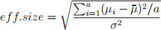
where µi , i = 1, 2, ..a = 4 true means of the four treatments and σ 2 is the true er-ror variance for the CRD that is being planned. Naturally you do not know these parameters which are needed to determine the number of replicates (n).
However, the researcher believes that the means and error variability will be very much similar to that obtained from her recently conducted CRD experiment. She thinks that it is appropriate to use the information contained in the CRD data given in file: ”DataHW2Q3F2023.csv”. [Hint: Analyze this dataset and obtain the estimates of µ ’s and σ 2 and use them for the parameter values.]
Obtain the minimum number of replicates using the following two approaches:
(a) [Points = 5] Use function pf() to compute the power. Here you may need to compute the noncentrality parameter, among other quantities. As there is no explicit expression for the number of replicates (n), you may repeat the power calculation for a range of values of n.
(b) [Points = 5] Using simulation and not the pf() function. In stead of computing the noncentrality parameter, you may generate the data on response variable from normal distributions with the µi ’s and σ 2 and the number of replicates (n). The dataset can be used to get information on these unknown parameters. You may use say number of simulation runs, say 5000 (you are free to use a larger number of runs.) In this case too, you need to compute the power for a range of values of n so that you capture the targetted power.
2023-10-21