MS 5217: Assignment 3
Hello, dear friend, you can consult us at any time if you have any questions, add WeChat: daixieit
MS 5217: Assignment 3
Due Monday 11:59 am, Oct. 16th.
1. Moneyball lite
We run a regression trying to understand the impact of OBP (on base percentage) on RPG (runs per game). The results for each team in the American League are shown below.
Coefficients:
Estimate Std. Error t value Pr(>|t|)
(Intercept) -8.247 1.921 -4.294 0.00104 **
OBP[League == "American"] 38.817 5.506 7.050 1.34e-05 ***
Residual standard error: 0.2099 on 12 degrees of freedom. R-squared: 0.8055.
(a) Verify the numbers in this table in R, using the baseball.csv data from the class website. Use the subset option in the lm() command to restrict the analysis to the American League teams.
(b) Give an approximate 90% confidence interval for the slope.
(c) Test the hypothesis that OBP is unrelated to RPG at the 10% level.
(d) What is the correlation between RPG and OBP?
(e) Give the plug-in 95% prediction interval for RPG when OBP is 0.400.
(f) Test the hypothesis that the true slope is exactly 30 at the 5% level. Count as extreme only values greater than the null hypothesis value of 30.
2. Below are the summary statistics for market returns and two mutual fund managers for 180 months. Suppose we assume stock returns have no serial correlation over time. Let’s use their summary statistics and CAPM to evaluate the performance for two mutual fund managers. You can use pnorm(), qnorm(), and dnorm() for the calculation.
Figure 1: Market Summary Statistics
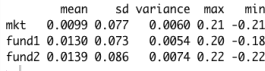
(a) Based on summary statistics in Figure 1, what is the probability for a 0.1 (or 10%) drop of market for a 2-month period? (Hint: sqrt(0.012) ≈ 0.1)
(b) Based on summary statistics in Figure 1, what is the probability for both Fund I and II lose 0.1 (or 10%) for a month if we assume their performance are independent?
(c) Based on CAPM regression results in Figure 2, could we tell if Fund I deliver a pos-itive alpha beyond the market? Please write down the null hypothesis and make your conclusion. (Hint: You are suggested to use 2 to approximate 1.96 for the calculation.)
Figure 2: CAPM Evaluation for Fund I and II
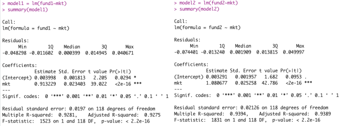
(d) Based on CAPM regression results in Figure 2, could we tell if Fund II has a market beta of 1? Please write down the null hypothesis and make your conclusion. (Hint: You are suggested to use 2 to approximate 1.96 for the calculation.)
(e) Based on above analysis, if the market drops 0.1 (or 10%) in September, what is the probability for both Fund I and II lose 0.1 (or 10%) for a month?
3. MidCity House Price
The MidCity.txt data set, available on the class website, contains data on 128 sales of houses in a midwest town over a given period of time. For each sale, the file shows an indi-cator of neighborhood quality, the number of offers made on the house, the square footage, whether the house is made out of brick, the number of bathrooms, the number of bedrooms, and the eventual selling price. Use regression models to estimate the pricing structure of houses in this town. Consider, in particular, the following questions.
(a) Should you include the Offers variable in the regression? Why or why not?
(b) Is there a premium for brick houses, everything else being equal? What is this premium, and does it change depending on which other variables you include? Why?
(c) Is there a price premium for houses in neighborhood 3 (those with a quality rating of 3)?
(d) Is there an additional premium for brick houses in neighborhood 3?
(e) Does combining neighborhoods 1 and 2 into a single category diminish the ability of the model to predict house prices as measured by the R2 ?
(f) Give a mean prediction and 90% plug-in prediction interval for a 1,500 square foot brick house with two bedrooms and two bathrooms in a nice neighborhood.
2023-10-16