487/819– Computer Vision and Image Processing Assignment 1
Hello, dear friend, you can consult us at any time if you have any questions, add WeChat: daixieit
487/819– Computer Vision and Image Processing
Assignment 1
Date Due: October 6, 2023, 6:00pm
Total Marks: 43
1 Submission Instructions
• Assignments are to be submitted via Canvas.
• Programs must be written in Python 3 within a Jupyter (iPython) notebook.
• Submitted notebooks must contain the results of the code when executed — the markers should not have to run your notebooks to generate output.
• Most assignments will require you to submit multiple files. Canvas doesn’t handle multiple files well. Add all of the files you are instructed to submit to a single .zip file, and submit that .zip
file. Only .zip files are accepted. Do not use 7zip or RAR format. We can’t unpack those.
• Absolutely no late assignments will be accepted. See the course syllabus for the full late assignment policy for this class.
The purpose of this assignment explore de-noising algorithms. As part of this assignment, you will implement a vector median filter since this filter is not available in the skimage library.
You have been provided with an images directory which contains some sub-directories, each of which contains a set of images. These images are used in both questions on this assignment. The contents of each sub-directory are described as follows:
noiseless: These are the original images, free of corruption from noise. These images are only to be used to compute PSNR and SSIM de-noising performance metrics. These images are used in questions 1 and 2.
noisy: These are noisy images corrupted with two different kinds of noise — additive noise and impulse noise. The severity of the additive noise differs from image to image. The impulse noise probability is the same for all images. These images are used only in question 2.
denoised: This empty directory serves as a place for you to save your de-noised images so that you can inspect them for correctness. This is provided only to help you stay organized, and it is up to you whether you choose to use it or not. It’s use is not required.
noisify.py: This is the script that was used to generate the noisy images from the noiseless images. It’s not necessary to use this file at all in your solution but if you want to know exactly how the noisy image were generated, you can look in here.
Note for users of Jupyter Lab on skorpio or trux: These images have already been placed on local storage on trux.usask.ca and skorpio.usask.ca. You do not need to upload them if you use jupyter lab on those servers. You can access the image folders containing the images as:
• /u1/cmpt487-819/data/asn1/images/noisy
• /u1/cmpt487-819/data/asn1/images/noisless
Moreover, the images.csv file can be found in the directory:
• /u1/cmpt487-819/data/asn1
You won’t be able to view these folders in the jupyter lab file browser because the server won’t let you look outside of your own home directory. But you’ll be able to access them from your script using these absolute paths. The contents of each folder are identical the corresponding folders you’ll see if you unzip the provided files on your own computer.
2.1 Assignment Synposis
In question 1 you’ll explore the de-noising performance of three different de-noising methods we discussed in class.
In question 2, you’ll first you’ll implement the vector median filter. Then you’ll use it to filter the provided noisy images, and obtain the PSNR and the SSIM of the noisy and median filtered images by comparing them to the noiseless images. The filtered images should have better PSNR and SSIM than the noisy images. Then you’ll develop a customized denoising algorithm for the provided noisy image dataset that can outperform the vector median filter alone and compare the PSNR and SSIM of the new algorithm to your previous results.
2.2 Implementing the Vector Median Filter (VMF)
Even though VMF isn’t the fastest operation, you can make it incredibly and unnecessarily slow in Python. I suggest an approach where you only use loops to iterate over the rows and columns of the input image. Computing the vector distances can be done without use of loops if we consider three powerful numpy functions: tile, transpose, and reshape.
Example 1
The function numpy.tile() makes a specified number of copies of a matrix along a specified matrix dimension.
|
u = np . array ([ 1 , 2 , 3 ]) |
|
|
# make 5 copies of u along dimension 0 ( rows ) , and 1 copy along # dimension 1 ( columns ) . # Copies can be made into the third dimension by adding another element to # the tuple in the second argument . v = np . tile (u , (5 , 1)) >>> v array ([[1 , 2 , 3] , [1 , 2 , 3] , [1 , 2 , 3] , [1 , 2 , 3] , [1 , 2 , 3]]) |
|
Example 2
The function numpy.transpose() swaps the dimensions of a matrix. A common example is the swapping of the first and second dimensions (rows and columns) of a matrix which is equivalent to a matrix transpose. The transpose function generalizes this to any combination of dimensions. As a further example, we can “rotate” vfrom the previous example, into the third dimension (imagine rotating the matrix into the page about an axis along the top matrix row) by swapping the first and third dimensions (dimensions in python are numbered starting at 0):
# The second argument specifies which dimensions should become
# the new dimensions 0 , 1 and 2. In this case , dimension 2 ( planes ) becomes
# dimension 0 ( rows ) , dimension 1 ( columns ) remains dimension 1 , and dimension 0 # ( rows ) becomes dimension 2 ( planes ) causing the matrix to " rotate " about a
# horizontal axis into the page . Now we get a copy of the vector
# [1 ,2 ,3] at each index in the third dimension . ( We need to use
# np .expand _ dims () on v first because v is a 2 D array ; it needs
# to be a 3 D array to allow us to transpose into the 3 rd dimension
# so expand _ dims (v , axis =2) returns an array of shape ( v . shape [0] , v . shape [1] , 1)) .
w = np . transpose ( np .expand _ dims (v , axis =2) , (2 , 1 , 0))
>>> w [: ,: ,0]
array ([[1 , 2 , 3]])
>>> w [: ,: ,1]
array ([[1 , 2 , 3]])
...
>>> w [: ,: ,4]
array ([[1 , 2 , 3]])
Example 3
The function numpy.reshape() takes an array and changes its width, height, and depth to new values provided that the product of these new values is equal to the product of the width, height, and depth of the input array (it can’t change the total number of matrix elements, just rearrange them). For example,if we take a sub-matrix of a larger image matrix (that might represent a neighbourhood!) that has dimensions 5 × 5 × 3, we can convert it into a matrix with 25 rows and 3 columns, where each row consists of the R G B values of one of the 25 pixels:
# get the pixels of the colour image I in a 5 x5 window centred on (r , c ) .
Iwindow = I [r -2: r +3 , c -2: c +3 , :]
# Reshape the 5*5*3 elements of Iwindow into a matrix of size 25*3 so # that each row of ’ colours ’ is the RGB values of a pixel in Iwindow .
colours = np . reshape ( Iwindow , [ IWindow . shape [0] * Iwindow . shape [1] , 3])
VMF Implementation Approach
To compute the median colour of a neighbourhood about (x, y), you will use tile, transpose, and reshape, to do the following. You will construct from the colour vectors in the neighbourhood about (x, y) two 3D matrices Y and X as described below. Assume there are n colour vectors in the neighbour- hood, e.g. for a 5 × 5 neighbourhood n = 25.
Construct the first matrix, Y, so that it has a depth of n, where each plane is equal to the n × 3 matrix of colour vectors in the neighbourhood of (x, y). This can be done with code similar to that given above, and a call to numpy.tile(). Thus each of the n planes of the resulting n × 3 × n array should look like this:

for 0 = 1 . . . n − 1 (n such planes extending into the third dimension) where v0, v1, . . . , vn−1 are the colour vectors in the neighbourhood. That is, row i of each plane of Y contains the RGB values of the one pixel colour in the neighbourhood and each plane is identical to the others.
Construct the second matrix X so that it also has n planes of size n × 3, but where the i-th plane contains n copies of just one of the colours in the neighbourhood, that is, ri, gi, bi:

Now, the difference between each plane of the two matrices can be used to compute the sum of the differences between the i-th colour and every other colour all at once! If you compute abs(X − Y) and sum the result over dimensions first two dimensions (rows and columns), you are left with a 1 × 1 × n matrix D where each entry D[0 : 0 : i] is the sum of the Manhattan distances (L1 norms) between the i-th colour and every other colour, which is just what we need for the vector median filter algorithm! The output colour for the neighbourhood is then the colour with the smallest sum of manhattan distance — find the index k of the minimum value in D, and the output colour for the neighbourhood should be Y[k, :, 0] = vk.
3 Problems
Question 1 (19 points):
Detailed instructions are provided asn1-q1.ipynb. Sample output for step 3 is given below.
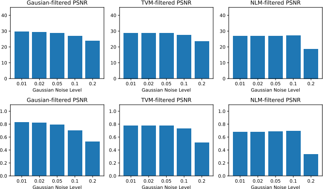
Sample Output for Step 2
The grading rubric is available on Canvas.
Question 2 (24 points):
Detailed instructions are provided asn1-q2.ipynb. Sample output for steps 2 and 3 are given below. These are the outputs from my solution. Depending on the de-noising algorithm you design, your value for the right-most bar in the bottom two graphs may differ, but the other bars should have the same height as shown here.

Sample Output for Step 2
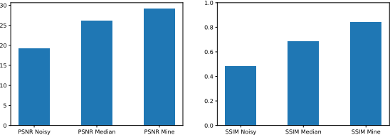
Sample Output for Step 3
The grading rubric is available on Canvas.
4 Files Provided
asn1-qX.ipynb: These are iPython notebooks, one for each question, which includes instructions and in which you will do your assignment.
Various Images in images.zip: As described in Section 2.
5 What to Hand In
Hand in your completed notebooks asn1-q1.ipynband asn1-q2.ipynb. Submitted notebooks must be executed prior to submission and contain the output of the code — the markers should not have to run your notebooks to generate output and will only grade the output that is submitted.
2023-09-26