ELEC2103 Tutorial 6 – Symbolic Mathematics and Nonlinear Equations 2021
Hello, dear friend, you can consult us at any time if you have any questions, add WeChat: daixieit
ELEC2103 Tutorial 6 – Symbolic Mathematics and Nonlinear Equations
2021
This tutorial is an introduction to the use of symbolic mathematics in MATLAB. It covers the creation of symbolic objects, the plotting of symbolic functions, the solution of algebraic equations.
6.1 Symbolic Objects
The Symbolic Maths Toolbox in MATLAB uses a special data type called a symbolic object which can be used to represent symbolic variables, numbers and expressions which can be manipulated according to the rules of algebra and calculus.
Help on functions of the Symbolic Maths Toolbox can be obtained in the usual ways. Some functions, such as diff, however, exist in a numeric and symbolic form. The command help diff gives help on the numeric version. For the symbolic version, use the command help sym/diff
6.1.1 Creating Symbolic Variables
Symbolic variables and expressions can be created using the sym function, for example:
x = sym('x') ;
a = sym('alpha') ;
creates two variables x and a which display as x and alpha respectively. If the variable name and the display string are the same, it is simpler to use syms. Thus
syms x y z
creates the three symbolic variables x, y and z.
Variables created in this way are complex. A symbolic variable can be constrained to be real. To create real variables x and y:
x = sym('x', 'real');
y = sym('y', 'real');
or, simply
syms x y real
6.1.2 Symbolic Numbers
Numbers can also be represented symbolically using sym. An example of converting to rational number form (other forms are possible):
x = sym(0.1) \% sym(0.1, 'r') does the same
thing
x = 1/10
y = sym(sqrt(5))
y = sqrt(5)
By default, the numbers are represented in rational form if such a form exists. (E.g. √ 5 cannot be represented in this way). Calculations can be carried out, using such representations, with infinite precision.
Other symbolic representations of a number are possible. For example
y = sym(sqrt(5),'d')
y = 2.2360679774997898050514777423814 is the value of √ 5 to 32 decimal digits. Th e number of digits depends on the setting of digits (default 32). To set the value to 10 digits:
digits(10)
y = sym(sqrt(5),'d')
y = 2.236067977
The function double can be used to convert a symbolic number to its normal numeric value.
z = double(y) \% z is a double, not a sym
object
z = 2.2361
6.1.3 Symbolic Expressions and Functions
We can create symbolic expressions and functions of symbolic variables, for example
syms t a b
f = sin(a*t+b)
f = sin(a*t+b) and operations such as differentiation (see later) can be carried out on them. Note that f is automatically cast as a symbolic object when it is defined in terms of symbolic variables.
For displaying symbolic expressions on the screen in a more readable form, the function pretty can be very useful. It displays expressions in a more readable form.
syms x
f = x^4+2*x^3−6*x^2+10
pretty(f)
f = x^4+2*x^3-6*x^2+10 4 3 2 x + 2 x - 6 x + 10
6.1.4 The Default Symbolic Variable
When an operation such as differentiation is performed on a function such as sin a ∗ t + b), it is often assumed that the differentiation should be carried out with respect to t. MATLAB does something similar. Thus, if the function diff is used to find the derivative of the function f above:
f = sin(a*t+b);
diff(f)
ans = cos(a*t+b)*a
This answer is as one might expect. But suppose we want the derivative with respect to a.
diff(f, 'a')
ans = cos(a*t+b)*t In the first case of the derivative, MATLAB uses the following rule to decide on the default symbolic variable: The default symbolic variable in a symbolic expression is the letter closest to ‘x’ alphabetically. If two letters are equally close, the later one is chosen.
The findsym function uses this rule to find the default variable:
findsym(f, 1)
ans = t
6.1.5 Plotting Functions
The fplot function can be used to plot symbolic functions. For details, use help sym/fplot. It will plot a function of one variable f(x) over the default range −5 ≤ x ≤ 5 with fplot(f). The range can be specified if desired. It will also plot an implicitly defined function f(x, y ) or a parametrically defined curve, i.e. f(x, y), with x and y functions of t, say. The usual functions such as axis, grid, etc, can be used to affect the resulting figure.
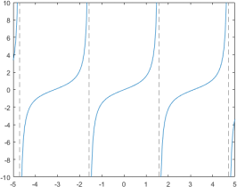
For example, if we wanted to use a symbolic form of the tan function for plotting, we could use the following:
syms x
y = tan(x);
fplot(y)
y = tan(x)
6.2 Getting Solutions
6.2.1 Simplification of Expressions
There are a number of functions which simplify expressions and carry out substitutions. They include collect, expand, factor and simplify.
The collect function collects all coefficients of a polynomial with the same power:
f = 2*x − 6 + x*(x^2 + 2*x − 7);
collect(f)
ans = x^3 + 2*x^2 - 5*x - 6
The expand function distributes products over sums and can do useful things to functions of sums:
f = a*(x+y);
expand(f)
ans = a*x + a*y
expand(cos(x+y))
ans = cos(x)*cos(y) - sin(x)*sin(y)
The factor function expresses a polynomial in terms of its factors (provided it can be done using rational numbers):
f = x^3 + 2*x^2 − 5*x − 6;
factor(f)
ans = (x+1)*(x-2)*(x+3)
The simplify function does general simplification including cancellation of common factors, application of trig identities, etc:
f = (x^3 − 3*x^2 + 3*x − 1)/(x − 1);
simplify(f)
ans = x^2 - 2*x + 1
simplify(sin(x)^2+cos(x)^2)
ans = 1
The simple function attempts to produce the form of expression with the fewest number of characters (not always the most useful result).
In gaining familiarity with these functions, a willingness to experiment is most useful.
6.2.2 Substitutions
Symbolic expressions do not have numerical meaning - they are just symbols (even if they look like numerical values, such as 1/3 or π they still of symbolic representations of them). In order to return numerical values from symbolic expressions, one first uses subs for symbolic substitution, where
subs(s,old,new)
returns a copy of s, replacing all occurrences of old with new, and then evaluates s. Note that even if subs replaces all of the symbolic variables in s with numerical values, then the returned value is still a symbolic numerical. For details, use help sym/subs.
(Also recall that to return numerical versions of symbolic numerical variables, explicitly recast the variables using double, which returns the variable as MATLAB’s standard double-precision float, or cast to another numerical type of your choosing.)
f = (x+y)^2 + 3
f = (x+y)^2 + 3
x = 5;
y = z^3;
subs(f)
ans = (5+z^3)^2 + 3
Alternatively (and note the use of cell arrays here),
subs(f, {x, y}, {sym('5'), z^3})
ans = (5 + z^3)^2 + 3
Other examples:
subs(f, 2) % substitutes for default
variable x
subs(f, y, (a+z)) % substitute for y
ans = (2+y)^2 + 3 ans = (x + a + z)^2 + 3
Exercise 1. A Lissajous curve, is the graph of a system of parametric equations:
x = A sin(at + δ), y = B sin(bt),
which describe complex harmonic motion.
(a) Write a script defining t, a, b and δ as symbolic variables.
(b) Assume A = B = 1 so they can be ignored, and then express the functions x and y above as symbolic expressions.
(c) Substitute in the following values: a = 1, b = 3 and δ = π/2 .
(d) fplot(x,y) can be used to plot parametric curves in two dimensions. Use this to plot the Lissajous curve defined above. Do you recognise this logo?
6.2.3 Solving Algebraic Equations
The solve function solves one or more equations for nominated variables. The simplest form simply accepts an expression as an argument, assumes the expression is equated to zero and solves for the default variable:
solve(a*x − b)
ans = b/a The following commands perform exactly the same task:
eqn = a*x == b;
solve(eqn);
\begin{lstlisting}
In these, you are defining an \textbf{equation} (not an expression).
This becomes an important distinction later when we consider systems of equations.
To solve for $a$ instead of $x$:
\begin{lstlisting}
solve(a*x−b, a)
ans = b/x
We can solve simultaneous equations as follows:
eqn1 = a + 2*b == 0;
eqn2 = 3*a − b == 5;
S = solve(eqn1, eqn2)
S = a: [ 1x1 sym ] b: [ 1x1 sym ]
S.a
S.b
ans = 10/7 ans = -5/7
Here, the solution is returned in the structure S which has fields a and b. There are two equations and two variables in this example, so there is no ambiguity about which variables to solve for. In other situations, you may need to specify the variables:
syms V E1 E2 s
eqn1 = V − E1 + V/3/s + (V−E)*s/4 == 0 ;
eqn2 = (E − V)*s/3 + E/4/s + E == 0 ;
S = solve(eqn1, eqn2, V, E);
S.E
ans = 48*E1*s^3/(84*s^3 + 84*s + 169*s^2 + 12)
Here, there are two equations in the four symbolic variables V , E1, E and s. A solution is carried out for V and E in terms of E1 and s, returning the structure S containing S.E and S.V, and the result for S.E is displayed.
Exercise 2. Use solve to find the values of x and y to 4 decimal places if:
x 2 + 10xy + 3y 2 = 15
y = 2x + 1
6.3 Calculus
A number of functions are available for performing calculus:
• diff (differentiation);
• int (integration);
• symsum (summation), and;
• limit (limits).
See help for details, the answer the following.
Exercise 3. Create the relevant symbolic variables and functions to determine the following:
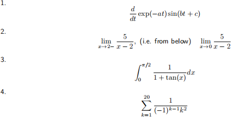
to four decimel places.
6.3.1 Descriptive equations for passive electrical components
Resistors, capacitors and inductors are a two-terminal, electrical components. They are the most fundamental passive components used in electrical and electronic circuits. In order to model them, we make use of some standard terminology. To start with, a component is a closed object from which at least two terminals emerge. A connection between two terminals is called a node, as we have seen in some previous weeks’ examples making use of graphs.
Beyond this we have a range of descriptive variables that describe the electrical behaviour of the components. These can be detailed electromagnetic variables, such as magnetic fluxes and electric charges, but these have the problem of not being measurable outside the boundary surface of the component in questions. They also interact on a scale this is often insignificant to the overall behaviour of the component and its interaction with other components in the circuit.
For this reason, in circuit analysis we typically focus on variables that are measurable at a component’s surface, namely voltages and currents, and derivative variables (electrical) power and energy.
Current A real variable i ∈ R, which, in general, depends on time: i = i(t). It is measured across the terminals of a component. The SI unit of measurement is the ampere,A.
Voltage A real variable ∈ R, which, in general, depends on time: v = v(t). It is associated with any pair of nodes in a circuit. The SI unit of measurement is the volt, V.
Power For a two-terminal component described by voltage and current behaviour, the absorbed electrical power is given by:
p(t) = v(t) i(t)
The SI unit of measurement of power is the watt, W. Note that the power delivered by a component is in the opposite sign to the power absorbed by it.
Energy The absorbed electrical energy of a component is defined as:

Note that the energy absorbed by a component can be
• converted or transformed into another form of energy, such as heat or mechanical energy, or
• stored as in an electromagnetic form (as potential energy in a magentic flux or electric field) or accumulated in another form (e.g. a battery stores energy in electrochemical form).
6.3.2 Capacitors
A capacitor is a passive two-terminal electrical component that stores potential energy in an electric field. To increase the energy stored in a capacitor, work must be done by an external power source to move charge from the negative to the positive plate against the opposing force of the electric field.
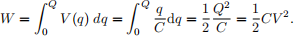
If the voltage on the capacitor is V , the work dW required to move a small increment of charge dq from the negative to the positive plate is dW = V dq. The energy is stored in the increased electric field between the plates. The total energy stored in a capacitor is equal to the total work done in establishing the electric field from an uncharged state.

where Q is the charge stored in the capacitor, V is the voltage across the capacitor, and C is the capacitance.
Exercise 4.
(a) In MATLAB, instantiate the integrand V (q) as a symbolic variable.
(b) A capacitor’s capacitance is defined as C = V Q , the ratio of charge to voltage. Rearrange this relationship write an expression for V as a function of C and (incremental) q.
(c) Using int, find W by integrating with respect to q from 0 to Q.
(d) Rearrange the capacitance definition again, this time with charge, Q, expressed as a function of voltage V and capacitance C, and substitute it into the integral you computed above, using subs. Report you answer; does it match your expectations?
Hint: You should have followed the standard derivation:
A similar derivation can be undertaken for inductors.
From next weeks’ lecture, we will begin to make use of symbolic differential operators to look at the time-domain response of these passive components to time-varying voltage and current sources, such as sinusoids and step changes.
2023-09-18