EECS 442: Computer Vision Fall 2023 Problem Set 2: Signal Processing
Hello, dear friend, you can consult us at any time if you have any questions, add WeChat: daixieit
EECS 442: Computer Vision
Fall 2023
Problem Set 2: Signal Processing
|
Posted: Wednesday, Sept. 13, 2023 Due: Wednesday, Sept. 20, 2023 Submission instructions: . Canvas:
– Colab notebook ( .ipynb) containing solutions and visualizations for 2.1(a-b), 2.2(b), 2.3(a). Also contains written solutions for 2.1(b) and 2.2(a). Before sub- mitting, please make sure to rename the file to <uniqname> <umid>.ipynb – .pdf version of Colab notebook. For your convenience, we have included the PDF conversion script at the end of the notebook. |

The starter code can be found at:
https://drive.google.com/file/d/1QN_Pxm1ha-NGUTJJcvyRekuzPmiCYuBs/view?usp=sharing
We recommend editing and running your code in Google Colab, although you are welcome to use your local machine instead.
Problem 2.1 Image blending
We will use Laplacian pyramids to blend two images.
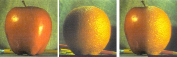
Figure 1: Blending with a Laplacian pyramid of 6 levels. Note that your result may look different than ours.
(a) (5 points) First, we will implement the following functions, which will be used to create a Laplacian pyramid from an image, and to reconstruct an image from a Laplacian pyramid.
You’ll recall that we’ll need to downsample in the Gaussian pyramid and downsample in the Laplacian pyramid. In your implementation, use Gaussian kernels for pyramid upsample and pyramid downsample
 . The kernel for pyramid upsample should be the same as the one for pyramid downsample, except that the kernel itself will be multiplied by
 4. (Hint: np.insert may come in handy when implementing pyramid upsample
 . Also, cv2.gaussianblur may come in handy when implementing pyramid.upsample and pyramid.downsample). Set the standard deviation of the Gaussian kernel as σ = 1.
. pyramid upsample
. pyramid downsample
Now that you can downsample and upsample your images, you can implement the Gaussian and Laplacian pyramids. (Hint: remember that you need the highest level of the Gaussian pyramid to start the Laplacian pyramid. See lecture slide #20 and #32)
. gen gaussian pyramid

. gen laplacian pyramid

Now that you can generate a Laplacian pyramid, you can reconstruct the original image with it. Use a Laplacian pyramid with 4 levels. Recall from lecture that, to reconstruct the original image, you repeatedly upsample the Laplacian (starting with the highest level of the Gaussian pyramid), and then add back the Laplacian from the next level of the pyramid . Please plot the original image, the Laplacian pyramid, and the reconstructed image. Also, numpy and cv2 libraries perform a clipping when subtracting images. Try to use a different method for image subtraction to make sure clipping doesn’t happen!)
. reconstruct img
(b) (2 points) Implement the function pyramid blend(im1, im2, mask, num levels)
 . Its inputs are two images and a binary mask (indicating which pixels to use from each image). The function produces a Laplacian pyramid with num levels levels that will blend the two
 image inputs. Use your function to blend the images of an orange and an apple that we provided in the Colab notebook. Plot the blended images with num levels ∈ {1
 , 2, 3, 4, 5, 6}. Please describe the difference between the blended images as the number of levels in the Laplacian pyramid varies: how does the result change as we increase the number of levels? Please include this in the cell in the .ipynb file, rather than uploading a separate document with a written answer.
To obtain color images, you can apply the blending to each color channel independently. In our implementation, this did not require any extra code (the same code worked on single-channel and multi-channel images due to numpy broadcasting). However, your implementation may differ.
(c) (Optional, 0 points) Use your code to blend your own images. If you would not like your blending results shown in class, please let us know!
Problem 2.2 Fourier Transform
(a) (1 point) Please match the images in the left column of Figure 2 to their corresponding spectrum visualization in the right column. Write your answers in a colon separated format (i.e. 1:A, 2:E, ...) in the provided cell in the .ipynb file.
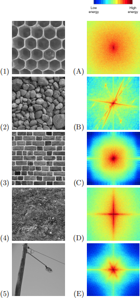
Figure 2: Images and DFT magnitude.
(b) (2 point) Convolve the provided image with a Gaussian filter: i) using direct convolution in the spatial domain, and ii) product in the frequency domain (via the convolution theorem). To perform DFT and inverse DFT, use fft2 and ifft2 from scipy.fft. For 2D convolution, we use scipy.signal.convolve2d. Note that doing this in the spatial domain versus the frequency domain might result in slightly different boundaries. That is okay for this problem!
(c) (Optional, 0 points) Show that complex exponentials are eigenfunctions of linear shift- invariant systems, i.e., if we convolve a complex exponential f[u] = ejwu with a filter g, we get a complex scaled version: f * g = (a + bj)f. (1 point)
Problem 2.3 JPEG image compression (Optional, 0 points)
The Central Campus dean has escalated his mysterious feud with the JPEG Standards Com- mittee: beginning next week, UMich will, by his order, be entirely JPEG-free. Fearing the huge increase in storage costs from dealing with uncompressed images, U-M ITS has created a simplified version of JPEG that they plan to deploy to all of their data centers over the weekend2 . They have turned to you for help in completing one small component of the system: the frequency decomposition.
JPEG image compression takes advantage of the fact that human vision is less sensitive to high frequency components than to low frequency components. It is therefore possible to discard some high frequency components without significantly reducing the visual image quality. In this problem, you will implement a variation of the Fourier transform called the discrete cosine transform (DCT), and explore it via simple visualizations. After implementing the DCT, you can plug it into U-M ITS’s new compression system to confirm that the model leads to significantly smaller images.
Note: Despite the large amount of code we have given you for the JPEG compression system (and the length of the question), this problem should only require a few lines of code!.
JPEG image compression can be divided into several steps:
1. Break the image into tiny 8 × 8 patches.
2. For each patch, apply the Discrete cosine transform (DCT) to obtain a frequency de- composition.
3. Quantization: high frequency DCT coefficients with small magnitude are set to zero.
4. Finally, we losslessly compress the quantized DCT coefficients. Since these contain a large number of zeros, they will compress much more easily than before quantization. This step uses Huffman coding (see here for more information, if you are interested)
Recovering the image from the encoded file follows the reverse of the above steps:
1. Decoding the Huffman-coded file to get the quantized DCT coefficients
2. De-quantization, where quantized DCT coefficients are scaled back to the actual scale
3. Inverse DCT to reconstruct the image.
By following the above steps, we will compress a grayscale image into a compact encoded file, examine its new file size, and then decode that compact file and reconstruct the image. You will implement the DCT transform part (step 1). We have implemented the remaining code for you. Please note that the amount of code that you’ll need to write is quite minimal!
Discrete Cosine Transform The DCT is very closely related to 2D Discrete Fourier Trans- form (DFT), which also describes how much of each frequency component an image contains.
It produces results that are entirely real-valued (rather than complex), and it is often better- suited to processing images than the DFT (see Szeliski 3.4.2 for more information) . The 2D DCT of an M × N matrix A is given by:

The values Bpq are called the DCT coefficients of A. The inverse 2D DCT is given by:

where in both (2) and (3), αp and αq are given by:

(a) (optional, 0 points) A core component of 2D DCT is the 2D DCT basis, which is a set of 2D sinusoidal images with different spatial frequencies of the form cos ![]() cos
cos ![]() . Implement function build 2D DCT basis that will compute this basis image set
. Implement function build 2D DCT basis that will compute this basis image set

 . Visualize the basis image set using the given code.3 (1 point)
(b) (Optional, 0 points) DCT 2D and IDCT 2D
 for performing 2D DCT and inverse 2D DCT are implemented using the built 2D DCT basis, read through the code of these two functions and make sure you understand them.
(c) (Optional, 0 points) Now, the full JPEG compression system should be ready to run! In the encoding part of the code, try image compression using different quantization tables, including dc only , first 3
 , first 6 and first 10
 . Each of these tables discards a different set of frequency components; tables that discard more components produce a more com- pressed, but lossier, image. For each quantization table, report the compress ratio (size of the compressed file divided by size of uncompressed file). Also, please briefly comment on their reconstructed image quality and file size, and explain why it is the case. (1 point)
Hint: Take a look at the function load quantization table and function quantize to un-
 derstand what they are doing.
(d) (Optional, 0 points) Read the Quantization and Huffman coding and decoding code if you want to understand JPEG more thoroughly. Try out the direct Huffman coding the image pixel values without DCT code block in the end. This will show that Huffman coding alone is unable to compress the image effectively.
2023-09-18