ECON 2300: INTRODUCTORY ECONOMETRICS Tutorial 1
Hello, dear friend, you can consult us at any time if you have any questions, add WeChat: daixieit
ECON 2300: INTRODUCTORY ECONOMETRICS
Tutorial 1: R and Basic Operations
At the end of this tutorial you should be able to
• use R to read, manipulate and save data and workfiles
• use R to compute descriptive statistics
• use R to conduct hypothesis tests concerning a population mean
Problems:
1. The text file consumption.txt contains observations on the weekly family consumption expenditure (CONS) and income (INC) for a sample of 10 families.
(a) Read the data into R.
(b) Draw a scatter diagram of CONS against INC.
(c) On checking the data, you find that your assistant has recorded the weekly consumption expen- diture for Family 8 as $900 instead of $90. Correct this error and redraw the scatter diagram.
(d) Compute the mean, median, maximum and minimum values of INC and CONS.
(e) Compute the correlation coefficient between CONS and INC. Comment on the result. (f) Create the following new variables
DCONS = 0.5CONS
LCONS = log(CONS)
INC2 = INC2
SQRTINC = √INC
(g) Delete the variable DCONS and SQRTINC.
(h) Delete everything.
2. At the Famous Fulton Fish Market in New York city, sales of whiting (a type of fish) vary from day to day. Over a period of several months, daily quantities sold (in pounds) were observed. These data are in the file fultonfish.dat. Description of the data is in the file fultonfish.def. Describe the first four columns.
(a) Use R to open the data file and name the series in the first four columns as date, lprice, quan and lquan
(b) Compute the sample mean and standard deviation of the quantity sold (quan).
(c) Test the null hypothesis that the mean quantity sold is equal to 7,200 pounds a day at the 5% level of significance.
(d) Construct the 95% confidence interval for part (c)
(e) Plot lprice against lquan and label the variable lprice as “log(Price) of whiting per pound” and lquan as “log(Quantity)” . Then, comment on the nature of the relationship between these two variables.
(f) Save this workfile to any folder on any drive.
ECON 2300: INTRODUCTORY ECONOMETRICS
Tutorial 1: R and Basic Operations
At the end of this tutorial you should be able to
. use R to read, manipulate and save data and workfiles
. use R to compute descriptive statistics
. use R to conduct hypothesis tests concerning a population mean
1 Introduction of R
1.1 Starting R
Before solving the problems, let’s look around the software R. If you have not yet installed R and RStudio, install them on your computer. There is an installation guide on the course webpage. Start R by double- clicking the icon of RStudio. On my computer (a Mac), the icon looks like:

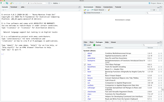
1.2 Opening Display
Once R is started a display will appear that contains a number of windows. Among them, Console is the most important and for the moment we will type R commands there. Another important window is Pack- ages, which shows a list of packages that are installed on the computer. Recall that a package is a collection of R functions and datasets, and R works with a number of R packages. We will use a few packages that have econometric estimators throughout the semester. The box next to ‘base’ is checked, which means the package called ‘base’ is loaded for use.
Moreover, across the top are R pull-down menus. We will explore some of them later. I encourage you should play around them.

We can check the current working directory (folder) by typing in
> getwd()
without “ >” (and hit the enter key) in the console window. In my case, R says that the current working directory is set to be (the rather lengthy and so I’ve replaced part of the path with an elipse ...)
[1] "C:/Users/uqrstrac/OneDrive -
All my folders are under that folder, and I don’t want to use the upper-most folder for this tutorial session. I will change the working directory to the folder where I want to save all files for this tutorial session. To do so, I type (the full path is rather lengthy and so I’ve replaced part of it with an elipse ...)
> setwd( "C:/Users/uqrstrac/ . . . /R tutorials/Tutorial01 ")
and I can check if the current folder is correctly set by using the command getwd(), which we used above. Of course, you should use a folder that exists in your computer, not the one shown above. Once you change the working directory, you can also see the list of files in the folder by typing
> list .files()
So far, we have used a few R commands: getwd , setwd , list .files. In particular, we used their very basic functions. When you need more functions, you can learn what’s available in the command using the help command. For example, try
> help( "getwd ")
and see what happens. Equivalently, try
> ?getwd
which I prefer, when I use R help, as it is simpler. Perhaps, help is the most frequently used command in R. I often find that Google is more useful to learn R (and other softwares, too). I will show you below how I learn R from the Internet.
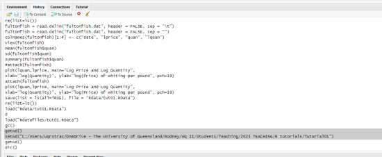
When you want to implement the commands that you have already used before, you can find them in the console window by pushing ↑ and ↓ buttons on your keyboard. Alternatively, look at the window on the top-right corner and click on the ‘history’ tab. Then, you will see the history of commands that you used so far. The history tab has its own functions,

which allow you to save/load the history, copy some of the commands in the history to somewhere else (like console), remove a part or all of the history, etc. Since how to use them is intuitive, you can learn by trying them and see what those functions do for you.
Alternatively, you can create your own script. Pull down the menu on the right-top corner.
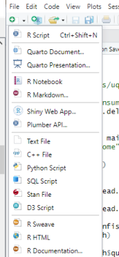
The menu gives you an idea that you can create documents in a number of different formats and also the programming in R can be interconnected to other languages like C++, Python, etc. (R is very flexible and powerful!!) For now, let’s just click on the first item, R Script. Then, an empty editor window (like a notepad) will pop up. You can type in your code in the editor. In my case, I go to the history tab, and selected the two lines as shown below;
Then, I click on "To Source" on the top of the history tab. Those two lines are pasted in the script;
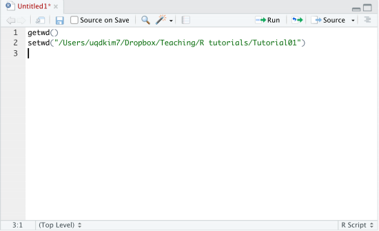
Then, place the cursor anywhere in the first line and click "Run". Then, R will run the command on the first line, getwd(). If you select more than one line and click "Run", R will implement the selected part of your script. Try! As you see on the top of the script window, the window has some other functions. For example, it is immediate that you can save the script for later use.
Now, before solving the tutorial problems, let’s close the current R session. Type in the console window
> q()
R disappears!
2 Answer Key for Tutorial 01
1. The text file consumption.txt contains observations on the weekly family consumption expenditure (CONS) and income (INC) for a sample of 10 families.
(a) Read the data into R.
(Answer)
When the datafile is in a text format, it is always a good idea to open it in a notepad to see the structure of the dataset. Just double-click on the file, consumption.txt. Then, a default soft- ware (e.g., TextEditor in Mac, Notepad in Windows) for text files will show the contents of the file;
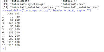
There are two variables and the first line has the names for them, CONS and INC. So, when we load the data into an econometrics software (not just R), we need to let the computer know that the first row is the header and the data starts from the second line. Also, the variables are separated by space. It could have been separated by other delimiters like commas, tabs, semicolons. We also need to let the computer know which delimiter is used in the raw data file.
Since it is our first time to use R, we do not know how to load a data file in R. Fortunately, R has a very (indeed very) large community of users and they exchange ideas, developing R and its packages, and answer each other’s questions. Therefore, it is very easy to find “how to” on the Internet. If you face a problem, there must be other people who already struggled the same issue. The answer should be there on the Internet. To learn how to load the file, for example, I google a few key words like R load data txt:
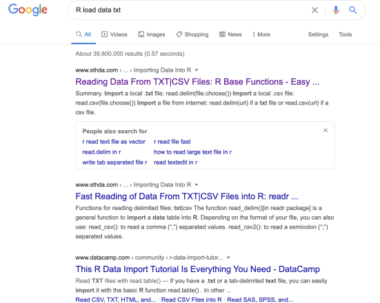
Then, I click on the first link, which opens (http://www.sthda.com/english/wiki/reading-data- from-txt-csv-files-r-base-functions) (← click this link!) that has a detailed explanation on how to open a text datafile. From this webpage, I can learn how to do the job;
> mydata <- read.delim("consumption.txt", header = TRUE, sep = "")
Using the R command read.delim I load the data in the file "consumption.txt" by informing R that the first line has the variable names (header = TRUE) and the variables are separated by space (sep = ""). Moreover, I create an R variable mydata to store the data. Now, you see that the data are stored in mydata in the ‘Environment’ tab in the top-right window. You have 10 observations and 2 variables in mydata.
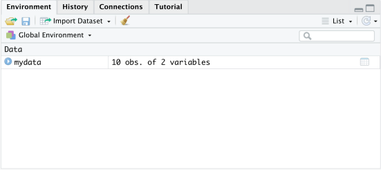
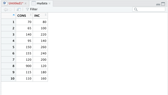
If you click on mydata in the Environment window, R will open another window to show a spread- sheet with the data.
We can keep exploring various functions in R. But, we will learn them by using R throughout the course. Let’s move on to the next problem.
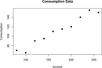
(b) Draw a scatter diagram of CONS against INC.
(Answer)
Again, I google a few key words like R scatter plot.
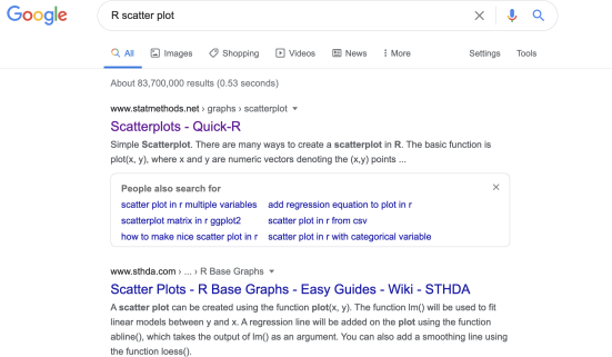
I choose the first one, (https://www.statmethods.net/graphs/scatterplot.html) ( ← click this link!) that explains in detail how to make a scatter diagram. As the webpage says, there are many ways to make a diagram in R. But, let’s try the simplest one:
> attach(mydata)
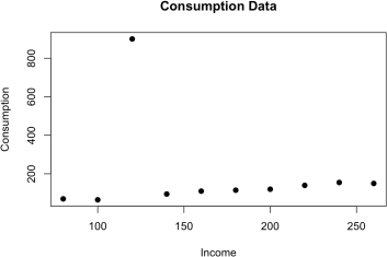
> plot(INC,CONS, main="Consumption Data",xlab="Income", ylab="Consumption", pch=19)
This generates the figure below. Note that without attaching the data, we should specify the dataset to which the variables belong in the command:
> plot(mydata$INC, mydata$CONS,
main = "Consumption Data",
xlab = "Income", ylab = "Consumption", pch = 19)
The command plot has several arguments. The first two are the X and Y variables. Then, it has options to choose a title (main) and labels (xlab and ylab) and the point style (pch).
Note that this diagram might be the simplest form in R. As the webpage explains R has many different ways to plot a diagram, providing a rich set of styling options. Look through the webpage above.
(c) On checking the data, you find that your assistant has recorded the weekly consumption expen- diture for Family 8 as s900 instead of s90. Correct this error and redraw the scatter diagram.
(Answer)
In the console window, type > mydata. Then, you will see
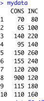
The data are in the form of a matrix whose (8,1) element has the error. So, we assign the correct value to it:
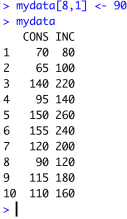
And then redraw the scatter diagram by repeating the command above.
![]() (d) Compute the mean, median, maximum and minimum values of INC and CONS. (Answer)
(d) Compute the mean, median, maximum and minimum values of INC and CONS. (Answer)

(e) Compute the correlation coefficient between CONS and INC. Comment on the result. (Answer)

The command cor() gives a correlation matrix. The off-diagonal elements are correlation coef- ficients between the variables indicated in the rows and columns. In this example, we have only two variables, which gives only one correlation coefficient (0.981). Since the correlation coefficient is close to (positive) one, consumption and income are moving in the same direction and they are closely related.
(f) Create the following new variables
DCONS = 0.5CONS
LCONS = log(CONS)
INC2 = INC2
SQRTINC = √INC
(Answer)

When we define a variable we can use both = and <- in R. Now, you have four additional variables in the Environment.

(g) Delete the variable DCONS and SQRTINC.
(Answer)
Try
> rm(DCONS,SQRTINC)
and check the Environment.
(h) Delete everything in the workspace.
(Answer)
Try
-> rm(list=ls())
and check the Environment.
Alternatively, click on the broom of the Environment tab.

2. At the Famous Fulton Fish Market in New York city, sales of whiting (a type of fish) vary from day to day. Over a period of several months, daily quantities sold (in pounds) were observed. These data are in the file fultonfish.dat. Description of the data is in the file fultonfish.def. Describe the first four columns.
(a) Use R to open the data file and name the series in the first four columns as date, lprice, quan
and lquan.
(Answer)
The data are in .dat format, which is not really familiar. To see what is in the file, I try to open it using a TextEditor (notepad).

The datafile does not have a header (variable names) but the fifteen variables are all nicely aligned as if they are separated by tab. So, I try to load the data and save it in the R object "fultonfish";
>fultonfish=read.delim("fultonfish.dat",header= FALSE,sep= "\t")
where the last option is used for tab delimiter. The environment tab, however, says that there is only one variable.

Something is wrong! So, I clear the workspace using the broom and reload the data but this time specifying the delimiter to be space.
![]()
Then, the environment indicates that there are 15 variables, as desired. By clicking on data item in the environment tab, we can see the data in a spreadsheet.

R gives variable names V1, V2, ... when the variables do not have a name. Now, we will give proper names to the first four variables. If you google a few relevant key words like change variable names, you will see that there are a few different ways of doing this. Some of them are using a package. Typically, a package is used when it simplifies the task. Since what we need to do is simple, let’s do it just without installing any new packages. Try:
![]()
Apparently, the command colnames is used for changing the names of columns and it takes the R object as an argument, which is fultonfish in this problem. Also, [1:4] chooses the columns (from the first to the fourth). Then, the rest is the way of giving names in R. Try >?c to learn more about c. Moreover, the command View(fultonfish) does the same job as clicking on the data item in the environment tab.

(b) Compute the sample mean and standard deviation of the quantity sold (quan). (Answer)

(c) Test the null hypothesis that the mean quantity sold is equal to 7,200 pounds a day at the 5%
level of significance.
(Answer)
Using the sample mean and standard deviation we obtain above, we can test the null hypothesis. The null is H0 : µ = 7, 200 and the alternative is H1 : µ ![]() 7, 200.
7, 200.
Since
![]() 'Xn - µ0 ' '6, 334.667 - 7, 200'
'Xn - µ0 ' '6, 334.667 - 7, 200'
' ˆ(σ)/^n ' ' 4, 040.12/^111 '
we reject H0. By the way, how do you know the sample size is n = 111?
Alternatively, we can do the test using a R command:

□
(d) Construct the 95% confidence interval for part (c)
(Answer)
6, 334.67 干 1.96 x 4040.12/^111 = 6, 334.67 干 751.58
Note that t.test( ) gives the 95% confidence interval too.
□
(e) Plot lprice against lquan and label the variable lprice as “log(Price) of whiting per pound” and lquan as “log(Quantity)” . Then, comment on the nature of the relationship between these
two variables.
(Answer)
Run the command below after attaching the data.
![]()
If you do not attach the data, you should specify the dataset to which the variables belong; see Q1(b).

(f) Save this workfile to any folder on any drive.
(Answer)
I will save everything in the current workspace in RData format. I will put it in the subfolder RDatafiles. I first create a subfolder in the current working folder and name it RDatafiles:

Then,
> save(list = ls(all=TRUE), file = "RDatafiles/tut01.RData")
Then, you will see there is a file tut01.RData in the folder RDatafiles. Later, when you need it, you can open the RData file and continue to work on the project. To see how to do so, let’s clear the workspace.
> rm(list=ls())
Load the RData file by
> load("RDatafiles/tut01.RData")
2023-09-15
R and Basic Operations