CONTROL M (ENG5022) 2016
Hello, dear friend, you can consult us at any time if you have any questions, add WeChat: daixieit
CONTROL M (ENG5022)
14th December 2016
SECTION A
Q1.
(a) State the Nyquist sampling theorem. Given a sampling time T, what is the
shift in frequency between two aliased harmonics ![]() 1 and
1 and ![]() 2 ? [5]
2 ? [5]
(b) Consider a continuous signal R(z) with the following qualitative spectral content:

|
|
|
Sketch the magnitude of the same signal after sampling, |
|
|
(c) |
Describe a workaround to prevent aliasing to occur, assuming that you cannot alter the sampling frequency |
|
|
(d) |
Sketch the spectral content of the sampled signal again, when the workaround is in place, showing and explaining how aliasing is prevented. [6] |
|
Q2 |
(a) |
Draw the structure of a two-degree-of-freedom feedback controller. Show the different signals, including disturbances, and explain their physical meaning. [4] |
|
|
(b) |
What are the three terms of a PID controller? Give the control law in the time domain and in the Laplace domain. [4] |
|
|
(c) |
What is controller design by pole assignment and how can this method be used to design a controller in transfer function form, C(s) = |
(d) In the state space description
̇(x)(t) = Ax(t) + Bu(t)
y(t) = Cx(t) + Du(t)
what is the requirement in terms of the properties of the matrices / vectors A, B, C and D for which the system is stable. What are the corresponding requirements for a transfer function G(s). [5]
SECTION B
|
Q3 |
(a)
(b) (c) |
The following transfer function is a lag network designed to increase the steady-state gain by a factor of 10 and have negligible phase lag at Φ1 = 3 rad/s : 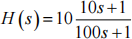 Find the gain (in dB) at Φ1 . Assuming a sample time T = 0.25 s, calculate the Nyquist frequency Φn . [2] Design the discrete equivalent of H(s) using the backward rectangular rule. [4] Compute the discrete equivalent of H(s) using the pole-zero matching technique (match the steady-state gain). [10] |
(d) Find the gain (in dB) at Φ1 of the discrete equivalents, and compare with that of H(s). [4]
|
Q4 |
(a)
(b) (c) |
The following transfer function is a lead network:  Find the discrete equivalent of it, when preceded by a zero-order hold (ZOH), for sample time T = 0.25 s. Use 4 significant digits for all numbers in the solution. [8] Using the inverse z-transform, find the corresponding difference equation. [4] State a necessary and sufficient condition for BIBO stability and determine whether the difference equation is BIBO stable. [8] |
Section C
Q5 A pendulum can be described by the following differential equation:
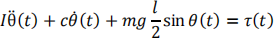
where θ(t) is the pendulum angle, τ(t) is an external applied torque, g is the gravitational constants, C is the damping coefficient, m is the mass, I is the inertia and l isthe length of the pendulum.
(a) Derive the linear transfer function in the s-domain for this model, considering the angle θ to be the output, and the external torque τ to be the input. You can assume that the angle θ is small. For the resulting transfer function, show how the natural frequency 幼n and the damping ξ depend on the physical parameters of the pendulum. [5]
(b) Calculate the transfer function of the pendulum plant, P(s), for the following physical values: m = 5kg, I = 0.2kgm2 , l = 0.4m, C = 0.5Nms/Tad, and g = 9.81m/s2. What are the values of 幼n and ξ? [3]
(c) Figure Q5 shows the Bode frequency response plot of the plant transfer function P(s) derived in (b).
(i) Discuss properties of the time domain response (such as steady-state gain, under- or over-damped response, frequency of any oscillations) which can be derived from this Bode plot. [3]

(ii) Consider a standard feedback control structure with a proportional
controller C(s) = 100. Calculate the loop gain L(s) and sketch the Bode plot of its frequency response, based on the plot shown in Figure Q5. Comment on the characteristics of the closed loop system (such as steady state gain/error, bandwidth, stability margins and damping) which you can derive from the plot of L(s) . [4]
(iii) The controller is amended by a derivative term CD (s) = 100 ![]() , so that the new PD controller is C(s) = 100 + 100
, so that the new PD controller is C(s) = 100 + 100![]() . How does the loop gain L(s) change, and what is influence of. this term on the characteristics of the close loop (such as steady state gain/error, bandwidth, stability margins and damping)? For your answer you should sketch the approximate frequency response of L(s), based on the frequency response of the modified C(s). [5]
. How does the loop gain L(s) change, and what is influence of. this term on the characteristics of the close loop (such as steady state gain/error, bandwidth, stability margins and damping)? For your answer you should sketch the approximate frequency response of L(s), based on the frequency response of the modified C(s). [5]
Q6
(a) Derive the closed-loop equation relating the plant output y and the plant input u to the signals r, d, and n. [2]
(b) Define the sensitivity function S0 and the complementary sensitivity function T0. Sketch the typical plots of |S0 | and |T0 | against frequency, based on the assumption that the plant has a low-pass character. [5]
(c) Describe the design goals which one attempts to achieve when designing closed-loop feedback systems. Describe factors which limit the extent to which these goals can be achieved. Relate your answer to the typical shapes of the sensitivity and complementary sensitivity functions. [7]
(d) Explain what is meant by the vector margin, sm , of a feedback system. Derive an expression linking the vector margin sm of the closed-loop system to the peak magnitude of the sensitivity function So. What is the equivalent expression linking the complementary vector margin Tm of the closed-loop system to the peak magnitude of the complementary sensitivity function To? Discuss why peaking of |S0 | and |T0 | should be avoided. [6]
2023-09-15