Hello, dear friend, you can consult us at any time if you have any questions, add WeChat: daixieit

School of Mathematics and Statistics

MAST90083: Computational Statistics and Data Science

Assignment 1

Question 1: Single and Multiple Linear Regression

This question helps you learn how to uncover the relationship between the predictors and a response variable. In case of linear regression, however, this relationship would be overfitted because all predictors will try to explain the response even those that have negligible effect on the response. For this question you need to call two libraries ”MASS” and ”ISLR”. We are going to use Boston dataset for this question. You can familiarize yourself with this dataset using these commands ”names(Boston)” and ”?Boston” before attempting this question

1. Using ”lm” function and Boston dataset in R fit a linear model for ”medv” using ”rm” as a predictor, for instance if medv is stored as a response in variable y and rm as a predictor in x then fitted data can be obtained as ”y.fit=lm(y ~ x,data=Boston)”. Both ”medv” and ”rm” are variables from Boston dataset.

2. Use ”plot” command for plotting the response variable (medv) against the predictor (rm) and ”abline” for plotting the fitted data. Do you see the linear approximation by fitted data?

3. A summary command on variable ”y.fit” will produce a ”Multiple R-squared” value of 0.4835. Can you find any other variable in Boston dataset (other than ”rm”) that can produce higher ”Multiple R-squared” than 0.4835. You must use correlation function on Boston dataset to suggest a solution. You may want to use library ”corrplot” for this purpose. Now, confirm your result by using the selected variable for linear fitting and then taking the summary of this new fitted data, and what is its multiple R-squared value?

4. Repeat the linear fitting from part 1 for all variables in Boston dataset and store it in y.mf it and then take a summary. From the summary table you can find the p-value (Pr(< |t|)) in right most column, using this can you suggest four variables that are enough to predict ”medv”?

5. Now plot Boston dataset using command ”plot(Boston)”, from this plot you must suggest which variable has minimal effect on ”medv”? Can you also suggest which variable has literally no role to play in this dataset? You can also see the value of the coefficients by using function ”coef(y.mf it)”, did you notice least square’s weakness has clearly been signified as it has ended up selecting all variables and even that variable that has a very weak effect on ”medv”? You may also want to use correlation matrix again on Boston data to get a clearer picture about this mystery variable.

Question 2: Ridge Regression and Lasso Regression

This question presents a way to resolve the issues with linear regression by doing variable selection so that predictors that fail to significantly explain the response can be dropped. However you will find that ridge regression although penalizes the coefficients, still fails to do variable selection because it together shrinks all of the coefficients towards zero. Lasso on other hand resolves this issue and only shrinks the insignificant coefficients towards zero. For this question we are going to use Hitters dataset

1. Load the Hitters dataset. Remove all those rows from Hitters dataset that have entry NA in the ”salary” column

2. For a design matrix construction, use function ”model.matrix” to read all variables in Hitters dataset excluding the salary and store them in variable x. Also, read the salary variable and store it in variable y. Generate a sequence of 100 values of λ between 10¹⁰ and 10^-2 and call the function ”glmnet” from glmnet library. You can generate the sequence as 10Λseq(10, −2, length = 100), where Λ is a ”raised to” sign. For glmnet, set α = 0, and estimate ridge coefficients for 100 λ values. Then, observe the set of coefficients for two extreme values of λ i.e. 10¹⁰ and also for 10^-2. For which value of λ among these two, the coefficient values are more close to zero?

3. Now, draw a plot of l2-norm of coefficient values (excluding the intercept’s coefficient value) against the logarithm of the λ values. Can you say from this plot that you cannot really decide the optimal λ value between 10¹⁰ and 10^-2 , better is to use the mean square error (MSE) plot against the λ values? Explain how can you say that?

4. The glment library already has a function ”cv.glmnet” that performs ten fold cross validation (CV). You are going to use this function to select an optimal λ. Now, first you need to set the seed equal to 10 for random number generator. Then randomly pick 131 samples from x for all variables and also the corresponding samples from y to construct a training dataset. The rest of the samples can be saved for testing dataset. Using this training dataset, plot the cross validation results, and find the best λ (the one that results in smallest CV error) value and its corresponding test MSE value (MSE value obtained using testing dataset and best λ), you may want to use ”predict” function here. Now refit the ridge regression model on the full data set using the λ chosen by CV. Examine the coefficients are they all present, similar to the linear regression case?

5. This time we set α = 1 (Lasso case) and again plot the cross validation results, and find the best λ value (using training set) and its corresponding MSE value (using testing set). Now predict the coefficients again using the best λ that we just selected. Were all coefficients selected again? Well most of them are zero, are they not?

Question 3: Model Selection

In this question we consider the analysis of three model selection criteria for selecting the order p of the following model

where ηt are independent identically distributed (i.i.d.) from N (0, σ²  ). The criteria we consider are

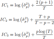
where .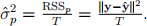

1. In the IC’s given above, T represents the number of effective samples. In the case of the model of order p above what is T?

2. Find the least square estimator of

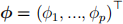
3. Provide the expression of

4. Generate two sets of 100 samples using the models

5. Using these two sets, compute the values of , and for p = 1, ..., 10 for models and . For each model provide a figure illustrating the variations of , and (plot the three criteria in a single figure for each model).

6. Using model generate 1000 sets (vectors) of size 100 and provide a table of counts of the selected model by , and

7. Using model generate 1000 sets of size 15 and provide a table of counts of the selected model by , and

8. Repeat questions 6 and 7 using model .

9. What do you observe from these tables?

10. Derive expressions for the probabilities of overfitting for the model selection criteria , and . For the derivation you will assume the true model to be p0 and consider overfitting by L extra parameters.

11. Provide tables of the calculated probabilities for M1 in the cases n = 25 and n = 100 with L = 1, ..., 8.

12. What are the important remarks that can be made from these probability tables?

13. The tables obtained from question 11 provide overfitting information as a function of the sample size. We are now interested in the case of large sample size or when n → ∞ (p0&L fixed). Derive the expressions of the probabilities of overfitting in this case.

14. What is the important observation that you can make?

Grading:

● Total: 20 points

● Question 1: 5 points

● Question 2: 5 points

● Question 3: 10 points

The assignment is to be submitted via LMS