ATOC20003 Atmospheric Modelling Assignment 2
Hello, dear friend, you can consult us at any time if you have any questions, add WeChat: daixieit
ATOC20003 Atmospheric Modelling Assignment 2
Due Thursday 31th August, 11:59pm on LMS
In this assignment, you will investigate numerical solutions to the 1D advection equation:

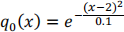
The initial conditions that you will use will be a single disturbance given by the equation:
Work through the three jupyter notebooks in order. The tasks that you need to need to do are indicated in the jupyter notebooks, but they are also repeated here.
Make all the plots indicated in the tasks, and answer the questions. Set out your report clearly, with headings for the three sections.
Part 1: Numerical solutions to the 1D advection equation [4 marks]
1. Plot the exact solution at the initial timestep, and at t=2 seconds
2. Run the two integration schemes, and plot both solutions after t=2 seconds together with the exact solution. The code is provided for the integration schemes! Your job is just to make the plots.
3. Insert the plots from (1) and (2) into your report, and answer the following question:
Which solution is 'better'? Consider that the disturbance (q) is a release of pollution, or an area of moist air. Are there some situations in which you would prefer one or other solution? [max 200 words]
Part 2: The impact of time-step and speed [8 marks]
In this part, you have been given each of the integration schemes as a function. The functions have the timestep, dt, and the advection speed, c, as inputs.
Your tasks are:
1. Test the functions for a range of different timesteps and advection speeds. Test timesteps between 0.02 and 0.18, in steps of 0.2. Test advection speeds between 0.6 and 1.6 in steps of 0.2.
2. Plot the outputs of the functions for a range of different timesteps and advection speeds. You should aim for two plots: one will show q(x,t=2) against x for the range of different
time-steps, and other will show q(x,t=2) for the range of different advection speeds. The
best way to do this is by using a for loop. If you choose not to use a for loop, then you need to be very systematic about the way you approach the task.
3. Insert the plots in your report. Discuss the results, and how they relate to the CFL criteria. [max 200 words]
Task 3: Assessing the quality of the solution [8 marks]
One way of determining how good a numerical solution is, is to consider the conservation of matter. For example, if q is a patch of pollution being advected along, then the total amount of pollution should stay the same, regardless of whether it has spread out. The numerical scheme should not create or destroy mass!
We can test this by integrating the total amount of pollution in the spatial dimension:
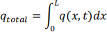
This expression can be written in python using:
qint[n] = np.trapz(q1, x=x_values)
This uses the trapezoidal numerical integration scheme. In this task, you're going to integrate the total q value at each step, to see whether the numerical integration is creating or destroying mass.
Your tasks are:
1. Run your functions, at output the total q at each time-step for each numerical scheme. Make plots of q against time.
2. Insert the plot from (1) into your report, and comment on the results. What are the
implications of this for numerical forecasts? What if q was moisture? [max 200 words]
3. (bonus 2 marks, up to a maximum of 20) Negative concentrations of q are impossible! One basic way of dealing with the fact the concentration fluctuates below zero, is to set any values of q that are less than zero to be exactly zero. Implement this correction into the leapfrog scheme, and re-calculate the total q as a function of time. What happens? Is this a good solution?
2023-09-05