The starter code can be found at:

https://colab.research.google.com/drive/1hsE0fNNvYPbjAmkId5IVi2gWOcmsx9oW?usp=sharing

We recommend editing and running your code in Google Colab, although you are welcome to use your local machine instead.

Problem 1.0 numpy review  (optional)

We will post a Colab notebook containing a brief introduction to numpy.  If you are new to numpy and numerical computing, we encourage you to work through these examples. They should cover the background that you need to complete this problem set. The Colab notebook can be found at:

https://colab.research.google.com/drive/1f7nAcXVy7jgvt21LhP_dHSmM-ARqUXCD?usp=sharing

Problem 1.1 Properties of convolution

Recall that 1D convolution between two signals f, g ∈ RN  is defined:

(a) Construct a matrix multiplication that produces the same result as a 1D convolution with a given filter. In other words, given a filter f, construct a matrix H such that f ∗ g = Hg for any input g. Here Hg denotes matrix multiplication between the matrix H and vector g (2 points).

(b) In class, we showed that convolution with a 2D Gaussian filter can be performed efficiently  as a sequence of convolutions with 1D Gaussian filters.  This idea also works with other kinds  of filters. We say that a 2D filter F ∈ RN×N  is separable if F = uv ⊤ for some u,v ∈ RN, i.e.

F is the outer product of u and v. Show that if F is separable, then the 2D convolution G * F can be computed as a sequence of two one-dimensional convolutions (2 points).

(c) (optional) Show that convolution is commutative, i.e.  f * g = g * f.  You may assume circular padding (e.g., f[−1] = f[N − 1]), zero padding, or whatever is convenient.  Note:  we will not grade this problem,  and you will not get  bonus points for completing it.

Hint: Write the equation for f * g, and figure out how to “rename” the variable used in the summation to arrive at g * f.

(d) (optional) Show that convolution is associative, i.e.  (f * g) * h = f * (g * h).

Note:   One  option is to define H  in  “bracket”  notation using  “...”   symbols,  e.g.,  H  =

lN  1   N  2   ...(...)   N1(−) 1].  Another option is to explicitly define the entries Hij .

Hint: Start by writing down the expression for G * F and then, inside the double summation, write F in terms of u and v.

(e) (optional) Show that cross-correlation,

is not commutative.

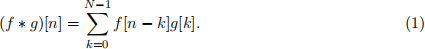
Figure 3:  (a) A pet photo helpfully delivered by our sponsor, (b) a failure case for a simple edge detector. These images are provided in the starter code. Photo credits can be found here.

necessary. Instead, implement the convolution as a series of nested for loops.  Compute the

edge  strength as Ix(2) + Iy(2) .  After that, create visualizations of Ix , Iy, and the edge strength,

following the sample code.

The filter response that your function returns should be the same dimensions as the input image. Please use zero padding, i.e. assume that out-of-bounds pixels in the image are zero. Also please make sure to implement convolution, not cross-correlation. Note that this simple  filtering method will have a fairly high error rate — there will be true object boundaries it misses and spurious edges that it erroneously detects.  The team at Petco, thankfully, has  volunteered to painstakingly fix any errors by hand (3 points).

Figure 2:  A meeting between the provost and a Petco representative, made using DALL-E 2.

(b) (Optional) This method detects edges fairly well on one of the dogs, but not the other.  Our sponsor would like us to investigate why this is happening. First, convert your gradient outputs to edge detections using a hand-chosen threshold τ (i.e. set values at most τ to 0 and those above to 1). Point out 2 errors in the resulting edge map — that is, edge detections that do not correspond to the boundary of an object — and explain what causes these errors.

(c) While the edge detector you submitted works well on some pets, engineers are reporting a large number of failures, and Petco higher ups are not happy.  Rumor is that it’s failing on pets that are playing in grass, especially for dogs with fluffy coats, such as “doodle” mixes — a particularly lucrative market for our sponsor (Figure 3b).  It appears that the gradient filter is firing on small, spurious edges.

Kindly address our funders’ problem by creating an edge detector that only responds to  edges at larger spatial scales.  Do this by first blurring the image with a Gaussian filter, before computing gradients. Implement your Gaussian filter on your own4 . Please do not use  any “black-box” Gaussian filter function for this, such as scipy.ndimage.gaussian filter .

Apply both the Gaussian filter and the gradient filter using a black-box convolution function scipy.ndimage.convolve on the image, rather than your hand-crafted solution.

(i)  Compute the edges without blurring, so we can look at the before-and-after results.

(ii)  Compute the blurred image using σ = 2 and an 11 × 11 Gaussian filter.

(iii)  Instead of blurring the image with a Gaussian filter, use a box filter (i.e., set each of the

11 × 11 filter values to 1/112).

(iv)  Compute edges on the two blurred images.

(v)  (Optional) Do you see artifacts in the box-filtered result?  Describe how the two results differ. Include your written response in the notebook.

Visualize the edges in the same manner as Problem 1.2(a).  Your notebook should contain edges that were computed using no blurring, Gaussian blurring, and box filtering. Please also show the two blurred images (2 points).