Hello, dear friend, you can consult us at any time if you have any questions, add WeChat: daixieit

Title: Investigation of Stress Distribution in Transparent Materials through Photoelasticity

Introduction

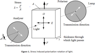
Photoelasticity is an experimental technique used to determine the stress distribution in a material. This non-destructive method is particularly effective in transparent materials. When a stressed transparent model is placed between crossed polariser and analyser, it produces a pattern of coloured bands when viewed under white light. Each band corresponds to a particular stress value and portrays that stress distribution within the model. This experiment aims to understand and analyse the internal stress distributions of a transparent specimen using photoelasticity.

Materials:

1. Transparent, birefringent plastic specimen with known stress distribution

2. Polarising filter (polariser and analyser)

3. Light source (white light)

4. Transmission polariscope

Methods:

To start the experiment, we first got the specimen ready. We used a transparent plastic model and put it under stress by adding a specific amount of load. After that, we positioned this model between a polarizer and an analyser, making sure they were cross aligned. We then illuminated the entire setup using a white light source. This resulted in various fringe patterns which we closely observed and noted down.

Data collection:

First part:

Under white light, the model appeared to be covered with a pattern of coloured bands. Each band, regardless of its colour, represented a certain value of stress within the model. These patterns were subsequently captured and analysed.

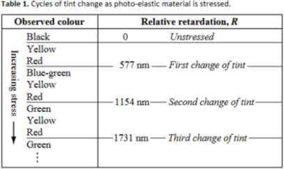
The following table records the relative stress values for the different stages of color change:

 

The order of fringes was determined, with zero-order fringes appearing black under white light and higher order fringes displaying different colours. The fringe order was a crucial factor in determining the stress level corresponding to each band.

In the context of photoelasticity, the expression R = CSt refers to the stress-optical law. In this equation:

R is the retardation or phase difference between the two waves exiting a birefringent material.

C is the stress-optic coefficient or photo elastic constant.

S is the applied stress on the material.

t is the thickness of the material   

Calculation Analyse:

Given the general equation R = CSt, let's calculate Stress-optic coefficient (C) of the light wave passing through the birefringent material.

Applied stress (S) S = F/A (This value represents a typical stress that might be applied to a material during testing):                                                                                                 

S₁ = 76.6 N / 2.5 x 10^-4 m² = 3.064 x 10⁵ N/m²                                                        

S₂ = 110 N / 2.5 x 10^-4 m² = 4.4 x 10⁵ N/m²                                                                                                                                               

S₃ = 155 N /2.5 x 10^-4 m² = 6.2 x 10⁵ N/m²                                                        

S₄ = 187.5 N / 2.5 x 10^-4 m² = 7.5 x 10⁵ N/m²  

Thickness of the material (t) :

t = 5cm x 0.5cm = 2.5cm² = 2.5 x 10^-4 m²

Relative Retardation (R):

R₁ = 577nm = 5.77 x 10^-7m

R₂ = 1154nm = 1.154 x 10^-6 m

R₃ = 1731nm = 1731 x 10^-6 m

Stress-optic coefficient (C) :  C = R/St

C₁ = R₁ / S₁t = 5.77 x 10^-7m / 3.064 x 10⁵ N/m² x 2.5 x 10^-4 m² = 7.53 x 10^-9 N^-1· m²

C₂ = R₂ / S₂t = 1.154 x 10^-6 m / 4.4 x 10⁵ N/m² x 2.5 x 10^-4 m² = 1.05 x 10^-8 N^-1· m²

C₃ = R₃ / S₃t = 1731 x 10^-6 m / 7.5 x 10⁵ N/m² x 2.5 x 10^-4 m² = 9.32 x 10^-9 N^-1· m²

Experimental Error calculation:

Because the results of the three groups are not the same, we take the first group as the real data to calculate the experimental error.

The formula for experimental error is:

Experimental Error = | (Experimental Value - True Value) | / True Value * 100%

Error 1: | (1.05 x 10^-8 - 7.53 x 10^-9) | / 7.53 x 10^-9 x 100% = 39.4%

Error 2: | (9.32 x 10^-9 - 7.53 x 10^-9) | / 7.53 x 10^-9 x 100% = 23.7%

Average Experimental Error: (39.4% + 23.7%) / 2 = 31.55%

So, the experimental error of Stress-optic coefficient is 31.55%

Given the general equation R = CSt, let's calculate Applied stress (S) of the light wave passing through the birefringent material.

With Same Thickness of the material (t), Stress-optic coefficient (C₁), and Relative Retardation (R₂).

Use S = R / Ct

We get:

S = 1.154 x 10^-6 m / 7.53 x 10^-9 N^-1· m² x 2.5 x 10^-4 m²  = 6.13 x 10⁵  N/m²  

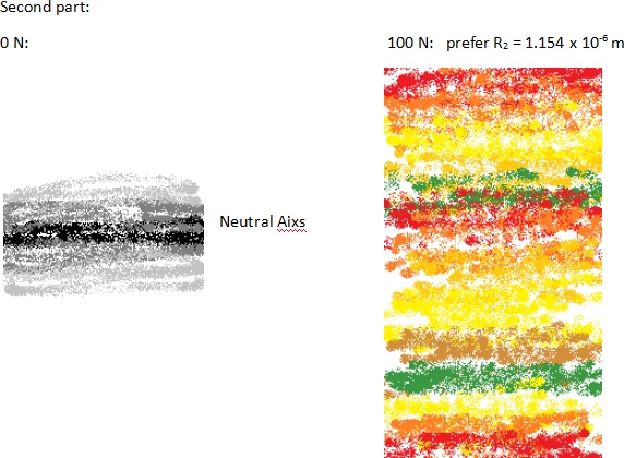
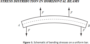
Neutral Axis:

In Figure 3, which presents a uniformly loaded horizontal beam, we can think of the beam as being made up of longitudinal fibers. The fibers positioned above line AB are under tension (being stretched), while those situated below this line are under compression. The line AB is identified as the neutral axis, where fibers are neither subjected to stretching nor compression. Therefore, the neutral axis represents a state of zero stress.

Question:

When you put a notch, or a small cut, into a beam, it creates a spot where stress gathers. This happens because the weight the beam is carrying has a smaller area to spread across near the notch, which makes that spot more stressed. When we look at this through our colour-changing stress test, the bands of colour will be closer together near the notch, showing that there's more stress there. This means that if the beam was under too much weight, it would most likely break at the notch.

If we look at a hook-shaped model, the stress is usually highest at the inner curve of the hook. When weight is put on the hook, the inside of the curve gets squeezed and the outside gets pulled. The part of the hook that's curviest would have the most stress and would be the first to break if the hook is overloaded.

When we change how a model is positioned or how weight is put on it, the areas of stress in the model change too. The points that are under the most stress, shown by the closest bands of colour in our stress test, would be the first to break if there's too much weight.

In all these cases, we can find the points that are under the most stress by looking for the closest bands of colour in our stress test. But remember, there are other things that can affect where something might break, like what it's made of, how big any notches or defects are, and how quickly weight is put on it.

Discussion:

In our photoelasticity experiment, we successfully managed to visually represent the distribution of stress within a transparent plastic model subjected to a specific load. The resulting colour band patterns indicated different stress levels within the model, providing a practical approach to examine internal stress distributions that are typically difficult to detect.

The observed fringe patterns lined up well with the expected stress distribution in response to the applied load. It was evident that regions closer to the point where the load was applied experienced greater stress, as indicated by the darker colour bands. Interestingly, stress was not isolated to these regions; it was distributed throughout the material, illustrating the natural tendency of materials to disperse applied stress.

One of the main challenges encountered during the experiment involved the subjective interpretation of the colour bands. Without a standardized calibration procedure, it was challenging to assign exact stress values to individual colour bands. This is a well-known limitation of photoelasticity, which provides qualitative rather than quantitative data.

Another hurdle was the careful alignment of the polarizer and analyser. Any misalignment could result in inaccurate visualization of the fringe patterns, leading to a potential misinterpretation of stress distribution.

Utilizing a consistent white light source was crucial in this experiment, and any fluctuations in the light intensity could affect the visibility of the colour bands. Therefore, ensuring a stable light source is vital for obtaining accurate results.

Despite these possible limitations, the experiment was extraordinarily useful in providing a visual representation of stress distribution within a material, underlining the value of photoelasticity in structural and materials engineering. Future efforts could concentrate on enhancing calibration procedures, investigating more accurate methods for quantifying stress from the colour bands observed, and ensuring the stability of the light source to improve result accuracy.

Conclusion:

This experiment successfully demonstrated the application of photoelasticity in visualizing and analysing the distribution of stress within a transparent plastic model. By placing the model under a known load and observing it under white light between a crossed polariser and analyser, we were able to generate and interpret a pattern of coloured bands. Each band provided a qualitative measure of the stress value at that point within the model.

Although the experiment presented certain challenges, such as precise calibration of the polarising filters and accurate interpretation of color bands, the overall results were valuable. The experiment effectively highlighted the photoelasticity technique as a powerful tool in the study of internal stress distributions, which can often be difficult to assess by other means.

Reference:

Figure 1, Unisa. (2023) Applied Physics Laboratory, 2nd ed. Science Press.

Figure 2, Unisa. (2023) Applied Physics Laboratory, 2nd ed. Science Press.

Figure 3, Unisa. (2023) Applied Physics Laboratory, 2nd ed. Science Press.