BX2022 Assignment 2 Template
Hello, dear friend, you can consult us at any time if you have any questions, add WeChat: daixieit
BX2022
Part A
Over the past decade, the United States’ percentage annual GDP growth has fluctuated between 0.82% and 2.39% (See appx. item A1). Over the same period, prices have increased between -0.36% and 3.16% (Appx. item A2). The current account balance has fluctuated between -2.88% and -2.08% of GDP (Appx. Item A3). Imports have fluctuated between 17.26% and 14.64% of GDP while exports have fluctuated between 13.54% and 11.72%; imports have exceeded exports in every year since 1975 (Appx. Item A4). Since 1970, government expenditure has exceeded taxation revenue in every year (Appx. Item A5).
Consumption is the greatest component of GDP, accounting for 81% since 1990; Investment accounted for 1%; Government expenditure 15%; Exports 11%; and Imports 14% (Appx. Item A6). Over the last 20 years,the Marginal Propensity to Consume averaged 0.67, Marginal Propensity to Import 0.24, and Marginal Propensity to Save 0.13 (Appx. Item A7).
Unemployment has been steadily decreasing since 2010, reaching 3.67% in 2019, which is the lowest level of unemployment since 1969 (Appx. Item A8).
Part B
Estimating the IS, LM and BP curves
IS Curve: The IS curve represents the set of pairs of the real interest rate and national income where the goods market is in equilibrium (where total production equals total expenditure and total investment equals total savings). When there is a movement in the interest rate, there is a change in planned investment, which influences total expenditure. The incremental expenditure generated by a change in interest rate is proportional to the multiplier, which is dependent on MPC; a higher (lower) MPC increases (decreases) the incremental expenditure and, therefore, national output, given the equilibrium condition, shown by a flatter (steeper) IS curve. Since the United States’ MPC of 0.67 is within the range estimated for Australia’s, the United States’ IS curve’s slope is likely similar to that of Australia’s (Berger-Thomson et al., 2009).
LM curve: Conditions for a liquidity trap to be present include a nominal interest rate which is near 0% and changes in the money supply being unable to affect prices (Krugman, 1998). The United States’ Federal Funds Rate has fluctuated between 1.4% to 2.5% p.a. in the past two years, which is probably not low enough to indicate a liquidity trap (Appx. item B1). Therefore, the LM curve will be upwards sloping.
BP curve: The United States probably has high capital mobility because capital controls were removed in 1974, liberalising capital flows internationally (Ghosh & Qureshi, 2016). However, it is unlikely that the United States has perfect capital mobility, since that would require the United States'financial assets to be perfect substitutes for foreign financial assets, which is unrealistic. Therefore, the BP curve must have a gradient greater than zero but be only slightly upwards sloping.
Drawing the IS-LM-BP model
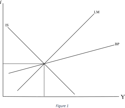
Given these characteristics deduced of the IS, LM and BP curves which model the United States’ economy, and assuming that the goods market, money market and balance of payments are in equilibrium, the following IS-LM-BP model [Figure 1] can be drawn:
Effect of price level on the IS-LM-BP model
As the price level decreases, the IS, LM and BP curves shift right, resulting in a higher equilibrium output level [Figure 2]. For the LM curve, this is because decreases in P increase the real money supply, meaning that at all levels of interest rate, money is willing to be supplied in greater amounts. For the BP curve, decreases in P result in higher NX, causing an increased current account, meaning that national income must increase to deteriorate the current account to equate the capital account, returning the balance of payments to equilibrium. For the IS curve, the higher NX causes a direct increase in total expenditure, meaning that production must increase in order to equate expenditure and maintain equilibrium in the goods market.
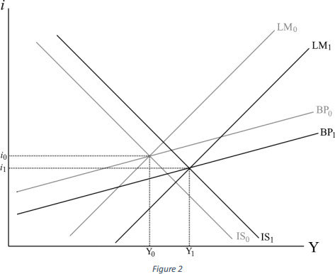
Hence, it is shown through the IS-LM-BP model that a decrease in the price level leads to higher real GDP. From this relationship, it is possible to derive an Aggregate Demand curve by plotting P and Y coordinates where the IS, LM and BP curves are simultaneously in equilibrium. Assuming that the IS0, LM0 and BP0 curves were taken at price level of P0 and the IS1, LM1 and BP1 curves were taken at a price level of P1, the Aggregate Demand curve [Figure 3] can be derived as:

It is presumed that the AD curve is steep (price-insensitive). This is because the US economy’s openness, as measured by exports and imports as percentages of GDP, is less than most countries, causing price changes to have lessened effects on GDP through movements in NX (OECD, 2016).
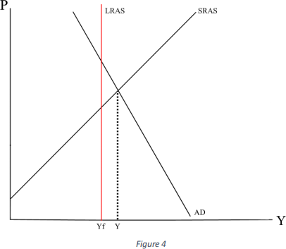
Next, short-run aggregate supply and long-run aggregate supply curves can be approximated to derive a complete AD/AS model of the US economy, which is presumed to be experiencing an inflationary gap [Figure 4].
Part C
Policy Recommendations
Low unemployment and inflation (3.7% and 1.8% respectively, appx. items A8 and A2) suggest that there is aslight inflationary gap, but the inflationary effects have not occurred yet. Therefore, contractionary policy will be employed.
The United States can be said to have a flexible exchange rate regime since the central bank in most circumstances allows the foreign exchange market to determine the US dollar’s exchange rates, rather than fixing the currency’s value (IMF, 2008). The exchange rate regime of a country alters the effectiveness of monetary and fiscal policies, since allowing changes to the exchange rate can shift the IS and BP curves.
Initially, contractionary fiscal policy [Figure 5] will shift the IS curve left. For example, if the government decreases expenditure, TE will be directly decreased, requiring Y to be reduced to maintain equilibrium in the goods market. As a result of the IS curve’s shift, the IS and LM curves will intersect at an interest rate that is too low for the BoP to be in equilibrium. This leads to a depreciation of the domestic currency, increasing NX, and therefore increasing TE and decreasing the CA deficit. The increase in TE shifts the IS curve right, while the decrease in the CA deficit shifts the BP curve right because less foreign investment (and therefore a lower interest rate) is needed to offset the CA.
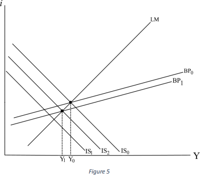
These shifts of the IS and BP curves lower the level of GDP at which the IS, LM and BP curves are simultaneously in equilibrium. The AD curve will be shifted left, reflecting that lower levels of real GDP will be demanded at all price levels. The SR and LR AS curves will not be affected [Figure 6]. Hence, contractionary fiscal policy can return the economy to its potential output without inflationary effects, and could be effective for a country with high capital mobility and flexible exchange rates like the United States.

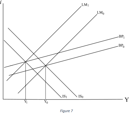
Contractionary monetary policy [Figure 7] initially shifts the LM curve left. This results in IS-LM intersecting above the BP curve, causing the domestic currency to appreciate. This leads to lower NX, decreasing TE and increasing the CA deficit. The lower TE shifts the IS curve left, while the increased CA deficit shifts the BP curve left. Therefore, the level of GDP when IS, LM and BP are simultaneously in equilibrium has been decreased. The AD curve is shifted left while the SR and LR AS curves are not moved [Figure 6], and contractionary monetary policy is effective for the US economy.
If a combination of monetary and fiscal policy were used, the subsequent shifts of the IS and BP curves due to movement in the exchange rate would depend on whether the initial shifts of the IS and LM curves from the stabilisation policy result in intersection of the IS-LM curves above or below the BP curve.
All the above policies could be effective at returning the economy to its potential output level.
However, contractionary fiscal policy is recommended because of its added benefit of reducing the budget deficit and hence the accumulation of national debt.
Bibliography
Krugman, P. (1998). It's Baaack: Japan's Slump and the Return of the Liquidity Trap. Brookings Papers
on Economic Activity, 1998, vol. 29, issue 2, 137-206. Retrieved from:
https://web.archive.org/web/20130524193008/http://www.brookings.edu/~/media/Projects/ BPEA/1998%202/1998b_bpea_krugman_dominquez_rogoff.PDF
Berger-Thomson, L., Chung, E. & McKibbin, R. (2009). Estimating Marginal Propensities to Consume
in Australia Using Micro Data. Reserve Bank of Australia. Retrieved from:
https://www.rba.gov.au/publications/rdp/2009/pdf/rdp2009-07.pdf
OECD. (2016). Trade in goods and services. Retrieved from:https://data.oecd.org/trade/trade-in- goods-and-services.htm
Ghosh,A., & Qureshi, M. (2016). What’s In a Name? That Which We Call Capital Controls.
International Monetary Fund. Retrieved from:
https://www.imf.org/external/pubs/ft/wp/2016/wp1625.pdf
International Monetary Fund. (2008). De Facto Classification of Exchange Rate Regimes and
Monetary Policy Frameworks. Retrieved from:
2023-08-30