1.    (a)  compute the directional derivative of f (x, g) = xg2 十 x3g at the point (4, -2) in

the direction u(^) =  (1, 3).

(b)  Find the equation of the tangent  plane to the surface z = f (x, g) = x2 十 g2 , at the point (1, 2, 5), in the form ax 十 bg 十 cz = d.

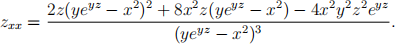
(c)  lf  x,g  and  z  are  linked  by  the  formula  ①2 z 十 g  =  eg从   determine  zx   and  zg  via implicit diferentiation and use (one of) these to show that

2.  cobb and Douglas (1928) deined their production function using data from the Amer- ican economy from 1899 to 1922, relating an output function Q = Q(k, L) to capital k and labour L, as follows

Q(k, L) = pkbLa

with itting coeicients p,  a and b.   using  modern  least-square  data  techniques,  for another economy with data from  1899 to  1922 we found that p = 0.8, a = 0.8 and b = 0.25.

(a) Assuming a cost function of the form c(k, L) = 山kk 十 山LL and assuming a stable economy in equilibrium (i.e. the economy is assumed to be at the stationary point), and given the 1899 (equilibrium) data with Q*  = 100, k*  = 100, L*  = 100 determine  山k , 山L   in  1899  and calculate the cost  (irst  as  formulas  and  second evaluated for the given values).  ln  1922, for Q*  = 240, k*  = 480 and L*  = 200, determine 山k , 山L  again and calculate the cost.

(b)  How well does the cobb-Douglas function it these data for Q (also give errors in percentages)?  (Hints:  1001.05  必 126 and  (480)0.25 (200)0.8  必 324.)  ls the proit maximised at these two equilibria?   calculate  the  Hessian  and analyse  it at the critical point.  Discuss the validity of the cobb-Douglas function.

(c)  lnterpret your results by comparing the relative changes of labour and capital costs, both as general formulas and for the particular values given, 山LL/c and 山kk/c , from 1899 to 1922.  (Hint: show that the answers only depend on a and b.)

3.   (a)  consider a general quadratic form Q(x) = xTAx for an n-dimensional vector x. The principle minor test (PMT) for a symmetric matrix A concerns the following rules:  (i)  lf det(A)  > 0 and all  LPMs  >  0 then Q is  PD;  (ii)  if det(A)  >  0, LPM1  < 0 and signs of LPMs alternate with order k, then Q is ND; etc.  complete this PMT classiication of rules for all cases, including the cases with det(A) = 0 (so concerning the PSD, NSD and lD cases).  Subsequently, for n = 2, consider Q(从, g) = a从2  + 2b从g + cg2   = a ((从 + bg/a)2 + (ca - b2 )(g/a)2 ), with a  0. Analyse the PMT for this quadratic form and prove that the PMT classiication (for n = 2, a < 0) is correct.

(b)  consider the cobb-Douglas production function

Q(从,g, z) = 从1/4g1/4z1/4

subject to the budget constraint h(从,g, z) = a从 + bg + cz - d = 0, where a,b,c, d are positive constants. State the Lagrangian

L(从,g, z) = Q(从,g, z) - λh(从,g, z)

and deine  λ .   Find the  maximum  (从* , g* z* ) of Q in terms of these constants. Hence, ind expressions for the maximum value Q*  and for the corresponding value λ*  of the Lagrange multiplier (in terms of a,b,c, d). check also that the NDcQ is satisied.

(c)  For the functions  compared in (c), take a = b = c = 1 and d = 3 and use that for those values the stationary point 从*  = g*  = z*  = 1 with Q*  = 1.  Derive the bordered Hessian of the Lagrangian deined above at this equilibrium by using that (here) Lxx  = Qxx , Lxg  = Qxg , etc.  Demonstrate in detail whether the proit is maximum at this stationary point, or not.

4.  consider the function f (x,g, 从) = x2g从2 subject to a single inequality constraint g(x,g, 从) =

3x+3g + 从 - 1 < 0, together with three NNc,s (non-negativity constraints) x,g, 从 > 0.

(a) what is the NDcQ? ls it satisied or not?

(b)  state the KT-Lagrangian L(-)(x,g, 从, λ) and derive the corresponding KT-equalities and inequalities for this problem from the  “standard” Lagrangian

L(x,g, 从, λ, μ1 , μ2 , μ3 ) = L(-)(x,g, 从, λ) + μ1x + μ2g + μ3 从

with multipliers λ, μ1 , μ2 , μ3  持 0 (Hint:  eliminate μ1 , μ2 , μ3 ). That is, derive that the KT-equalities are:

xL-从   =0,    gL-g  = 0,

从Lz  =0,    λL） = 0,

and also provide the accompanying inequalities.  calculate the KT equalities from the KT Lagrangian L(-)(x,g, 从, λ).

(c)  Derive the stationary points, including  (x* , g* , 从* ) = (2/15, 1/15, 2/5), and corre- sponding multiplier λ*  and ind out which stationary point is a maximiser.

(d)  using  the  standard  Lagrangian  of  the  problem,  also  derive  (and  complete)  the general bordered Hessian HB  for this problem:

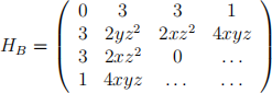
Show that evaluation at the critical point (x* , g* , 从* ) yields:

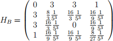
Given that LPM4   =  -64/28125,  LPM3   =  72/125 argue whether the  critical point is a minimum or maximum.