ECMT6006 Applied Financial Econometrics 2020 S1 Final Exam
Hello, dear friend, you can consult us at any time if you have any questions, add WeChat: daixieit
ECMT6006 Applied Financial Econometrics 2020 S1 Final Exam
Note: This is an open-book online exam. There are in total four problems and 25 questions. Please attempt all questions. The total mark is 50 and each question is worth 2 marks. You will have 2 hours and 30 minutes to answer the questions with handwritten solutions, and 30 minutes to scan and upload your solutions into Canvas.
Problem 1. [14 marks] Consider a two-period model for returns Rt, t = 1, 2 of an asset. Let ε0 = 1, and
Rt = µ + εt,
εt = σtνt, σt = |εt−1|,
where µ = 1, and ν1, ν2 are independent and identically distributed as
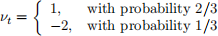
for t = 1, 2. Let Ft be the information set available at time t. Please answer the following questions.
(i) What is the probability distribution of R1?
(ii) What is the probability distribution of R2?
(iii) Compute the conditional mean E1(R2) := E(R2|F1).
(iv) Compute the conditional variance Var1(R2) = Var(R2|F1).
(v) Verify the law of iterated expectation E(R2) = E [E1(R2)] using numbers given in this problem.
(vi) What are the one-period ahead return point forecasts ˆRt for t = 1, 2?
(vii) What are the two standard deviation one-period ahead return interval forecasts for t = 1, 2?
Problem 2. [10 marks] Consider the following decomposition of the return of some financial asset:
Rt = µt + εt
where µt = Et−1(Rt) is the conditional mean of the return, and
εt = σtνt, νt|Ft−1 ∼ N(0, 1).
Answer the following questions.
(i) Show that εt is white noise process.
(ii) Show that ε2t is a conditionally unbiased proxy for σt 2 .
(iii) Consider the following “asymmetric volatility” model for the conditional variance:
σt 2 = ω + βσt 2 −1 + αε2t + δε2t−11{εt−1 ≤ 0}.
What empirical fact does this model try to capture? Explain why this model can capture this empirical fact.
(iv) The model in (iii) is estimated on daily returns on some empirical financial time series and the following results are obtained:
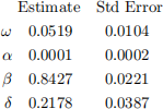
Describe how you would test whether the “asymmetric” term in this volatil-ity model is needed.
(v) How to construct the out-of-sample one-period ahead rolling window fore-casts of the volatility using this model?
Problem 3. [14 marks] Answer the below questions on the Value-at-Risk (VaR) and Expected Shortfall (ES) forecasting.
(i) Why VaR is often considered as a better risk measure than volatility?
(ii) Suppose a stock return follows a normal distribution with mean µ and variance σ 2 , i.e., Rt ∼ N(µ, σ2 ), for all t. What is the relationship between the 1% return VaR and the return volatility?
(iii) Explain the relationship and the major difference between VaR and ES. Why is modelling ES useful?
(iv) How to use the “Historical Simulation” (HS) model and the “Filtered Historical Simulation” (FHS) model to forecast 1% stock return VaR and ES?
(v) Which method (between HS and FHS) would you prefer to use in practice? Why?
(vi) How would you use the generalised Mincer-Zarnowitz regression to test whether the 1% return VaR forecasts from a model is optimal? Be explicit about the regression model, the null and alternative hypotheses, and how to test the null hypothesis.
(vii) Suppose you have obtained two VaR forecasts, V aRt HS +1 and V aRt FHS+1 for t = 1, . . . , T, from the Historical Simulation model and the Filtered Histor-ical Simulation model. How would you compare these two forecasts using the Diebold-Mariano test?
Problem 4. [12 marks] Let T be a set of a continuum of time. For any s ∈ T , consider the log asset price P(s) follow a continuous-time diffusion model
dP(s) = µ(s)ds + σ(s)dW(s)
where µ(s) is the conditional mean (drift) process, σ(s) is the instantaneous/spot volatility (diffusion) process, and W(s) is a standard Brownian motion. For any s ∈ T , let Fs be the information set at time s.
(i) For t1, t2 ∈ T and t1 < t2, let R(t1, t2) be the log asset return from time t1 to t2. What is the conditional distribution of R(t1, t2) given Ft1 ?
(ii) Let t = 1, 2, . . . denote the (discrete) number of days. Explain how to define the integrated variance IVt of the asset return on day t, i.e., from time t − 1 to t?
(iii) What is the difference between the integrated volatilty and GARCH-type volatility in terms of the risk measurement?
(iv) Denote Rt := R(t − 1, t) as the log return on day t. Prove the below relationship between the conditional mean of integrated variance IVt and the conditional variance of the log return rt:
E(IVt|Ft−1) = Var(rt|Ft−1).
(v) Explain how to estimate the integrated variance using intra-day asset prices.
(vi) Explain how the intra-day high frequency data can be used to build better volatility forecasting models. Please give specific examples.
2023-08-15