Homework Problems for Chapter 3
Hello, dear friend, you can consult us at any time if you have any questions, add WeChat: daixieit
Homework problems for chapter 3
3.1 properties of splines
(a). prove that the derivative of a quadratic spline is a irst-degree (linear) spline.
(b). show that the indeinite integral of a irst-degree (linear) spline is a second-degree (quadratic) spline.
3.2 working on splines
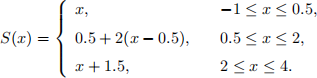
(a). Determine whether this function is a linear spline:
(b). Do there exist a,b, c and d so that the function
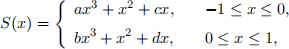
is a natural cubic spline?
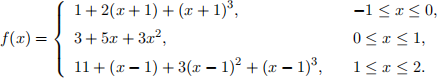
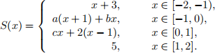
(c). Determine whether f is a cubic spline with knots -1, O, 1 and 2:
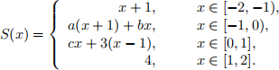
(d). Determine the values of a,b,c such that the following function is a linear spline.
(e). Determine the values of a,b,c such that the following function is a linear spline.
3.3 simple cases of Natural cubic spline
(a). Describe explicitly the natural cubic spline that interpolates a table with only two entries:

Here to , t1 are the knots. Give a formula for the spline.
(b). when the knots are uniformly spaced, i.e., hi = h for all i, natural cubic spline can be computed e伍ciently. Derive the simplest possible expression for the system in (3.4.5)

Find the matrix H and load vector yu.
(c). Determine the natural cubic spline that interpolates the function f (x) = x6 over the interval [O, 2] using knots (O, 1, 2).
3.4 constructing a Linear and a cubic spline.
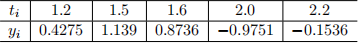
Given the data set:
a). Let L(x) be the linear spline that interpolates the data. Describe what L(x) consists of, and what conditions it has to satisfy. Find L(x), and compute the value for L(1.8).
b). Let C(x) be the natural cubic spline that interpolates the data. Describe what C(x) consists of, and what conditions it has to satisfy. In particular, set up the system of linear equations (3.4.5) (in text book, 2nd edition) or (3.4.12) (in text book, 1st edition). Find the spline function C(x), and compute the value for C(1.8). The computation here can be time consuming, and you may use Matlab to solve the system of linear equations.
3.5 大epresentation of Linear splines; (Bonus)
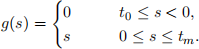
Given knots (to < t1 < . . . < tm). Deine a function g as
prove that every linear spline function with the knots (to , t1 , . . . , tm) can be written in the form
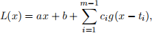
for a unique choice of the parameters (a,b, c1 , c2 , . . . , cm-1 ).
3.6 Linear spline in Matlab.
preparation. Read through the rest of“A PTactical IntToduction to Matlab”by Gock- enbach, at the web site
http://www.math.mtu.edu/~msgocken/intro/intro.pdf
your task. write a Matlab function that computes the linear spline interpolation for a given data set. You might need to take a look at the ile cspline-eval.m in section 3.4 for some hints on how to ind the index k such that ①k 三 t 三 ①k+1 .
Name your Matlab function lspline. This can be deined in the ile lspline.m, which should begin with:
function ls=lspline(t,Y,x)
X lspline computes the linear spline
X Ⅰnputs:
X t: vector, contains the knots
X Y: vector, contains the interpolating values at knots X x: vector, contains points where the lspline function
X should be evaluated and plotted
X Output:
X ls: vector, contains the values of lspline at points x
Here is a possible skeleton of a pseudo-code.
. Input: (t,y,x). output: L
. use a for-loop to go through each element of t(i)
— For each x(i), ind the integer K such that t(k) 三 ① (i) < t(k + 1);
— set L(i) to be the linear spline value.
. End of for-loop, then plot(x,L)
use your Matlab function lspline on the data set below:
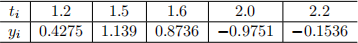
plot the linear spline for the interval [1.2)2.2], using at least 2OO points. This means, you may use x=[1.2: 0.01: 2.2].
what to hand in: Hand in the Matlab ile lspline.m, the script ile, and your plot.
3.7 Natural cubic spline in Matlab
The goal of this problem is to draw mount Everest with the help of natural cubic splines. we have a rather poor quality photo of the mountain proile, which is given below.
You need to set up a coordinate system, and select a set of knots along the edge of the mountain, and ind the coordinates for all these interpolating points. we are aware that the mountain proiles are not very clear in that photo, so please use your imagination when you ind these approximate points. You may either print out the mountain picture and work on it on a piece of paper, or send the image to some software and locate the coordinates of the interpolating points. Make sure to select at least 2O points. You may use more points if you see it.
After you have generated your data set, you need to ind a natural cubic spline inter- polation. use the functions cspline and cspline–eval , which are available in section 3.4. Read these two functions carefully, try to understand them before using them.
Does it look like there is a smaller peak on the right? Does the peak look rather sharp? How would you deal with this situation, knowing that a single cubic spline function will generate a “smoothest” possible interpolation?
what you need to hand in: A Matlab script that contains your data set, compute the spline functions, and draw the mountain. Also the plot of your mount Everest.
Have Fun!
3.8 Natural cubic spline with uniformly spaced 任nots
when the knots are uniformly spaced, i.e., hi = h for all i, natural cubic spline can be computed e伍ciently.
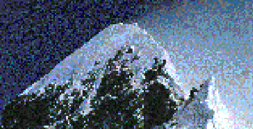
Figure 1: Natural cubic spline, for Mount Everest.
(a). Derive the simplest possible expression for the system in (3.4.5)
Hy从 = yu,
Find the matrix H and load vector yu.
(b). write a Matlab function, as simple as possible, to compute y从 for natural cubic spline interpolation with equally spaced knots. You may start with the given function cspline.m and simplify it, and make a function csplinesimple.m,
3.9 Interpolating a spiral with Natural cubic spline
consider the part of a spiral in 2D:
① (θ) = (θ/2 + 1) cos(θ), g(θ) = (θ/2 + 1) sin(θ), θ E [o, 1o].
In the ① - g plane, the spiral looks like:
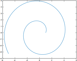
Taking the knots t = [o, 1, 2, . . . , 1o], interpolate the spiral segment with natural cubic spline, using the provided Matlab functions cspline and cspline-eval. plot the spline function and the data points together with the spiral, in diferent colors. How does the spline match the spiral? please comment on your result.
Turn in your Matlab script, the plot, and your comments.
2023-08-10