Question 1:

Task 1: High-frequency Finance (Σ = 30 marks)

The data file ‘IBM 202001.csv.gz’ contains the tick-by-tick transaction data for stock IBM in January 2020, with the following information:

Import the data file into Python and perform the following tasks:

1.1: Write code to perform the filtering steps below in the following order:                      (20 marks)

F1:  Remove entries that are outside the normal market trading hours,  i.e. before 9:30 am or after 4 pm

F2:  Remove entries with either transaction price, transaction size, ask price, ask size, bid price or bid size ≤ 0

F3:  Remove entries with bid-ask spread (i.e. ask price - bid price) ≤ 0

F4:  Aggregate entries that are (a) executed at the same date time (i.e. same ‘DATE’ and ‘TIME M’), (b) executed on the same exchange, and (c) of the same buy/sell indicator, into a single transaction with the median transaction price, median ask price, median bid price, sum transaction size, sum ask size and sum bid size.

F5:  Remove entries for which the bid-ask spread is more that 50 times the median bid-ask spread on each day

F6:  Remove entries with the transaction price that is either above the ask price plus the bid-ask spread, or below the bid price minus the bid-ask spread

Create a data frame called summary of the following format that shows the number and proportion of entries removed by each of the above filtering steps. The proportions (in %) are calculated as the number of entries removed divided by the original number of entries (before any filtering).

Here, F1, F2, F3, F4, F5 and F6 are the columns corresponding to the above 6 filtering rules, and Number and Proportion are the row indices of the data frame.

1.2:  Using the cleaned data from Task  1.1,  write  code  to compute Realized Volatility (RV) (defined in the lectures) for each trading day in the sample using 5min sampling frequency.  The required output is a Pandas series RVsr with index being the unique dates in the sample.        (4 marks)

1.3: Using the cleaned data from Task 1.1, write code to compute Two Time Scales Realized Volatility (TTSRV) for each trading day in the sample using the optimal sampling observations suggested by Zhang et al.  (2005) (see the lecture slides for more details).  The required output is a Pandas series

TTSRVsr with index being the unique dates in the sample.                                   (6 marks)

Task 2: Return-Volatility Modelling (Σ = 30 marks)

Refer back to the csv data file ‘SP100-Feb2023.csv’ that lists the constituents of the S&P100 index as of 8 February 2023 that was investigated in the group projects 1 and 2. Import the data file into Python.

Using your student ID or library card number (e.g.  12345678) as a random seed, draw a random sample of 2 stocks (i.e. tickers) from the S&P100 index excluding stocks ABBV, AVGO, CHTR, DOW, GM, KHC, META, PYPL and TSLA.1 Import daily Adjusted Close  (Adj Close) prices for both stocks between 01/01/2009 and 31/12/2022 from Yahoo Finance.  Compute the log daily returns (in %) for both stocks and drop days with NaN returns. Perform the following tasks.

2.1: Using data between 01/01/2009 and 31/12/2018 as in-sample data, write   code to find the best-fitted ARMA(p,q) model for returns of each stock that   minimizes AIC, with p and q no greater than 3. Print the best-fitted ARMA(p,q) output and a statement similar to the following for your stock sample.

Best-fitted  ARMA model  for  AMT:  ARMA(2,2)  -  AIC  =  8859.0599

Best-fitted  ARMA model  for  JPM:  ARMA(2,2)  -  AIC  =  11093.1840            (7 marks)

2.2: Write code to plot a 2-by-4 subplot figure that includes the following diag- nostics for the best-fitted ARMA model found in Task 2.1:

Row 1: (i) Time series plot of the standardized residuals, (ii) histogram of the standardized residuals, fitted with a kernel density estimate and the density of a standard normal distribution, (iii) ACF of the standardized residuals, and (iv) ACF of the squared standardized residuals.

Row 2: The same subplots for the second stock.

Your figure should look similar to the following for your sample of stocks.

Comment on what you observe from the plots.                                                     (5 marks)

2.5: Write code to plot a 1-by-2 subplot figure that shows the fitted conditional volatility implied by the best-fitted AR(p)-GARCH(p* , q* ) model found in Task 2.3 against that implied by the best-fitted ARMA(p,q) model found in Task 2.1 for each stock in your sample. Your figure should look similar to the following.

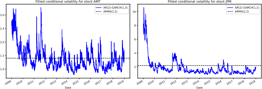
(5 marks)

Task 3: Return-Volatility Forecasting (Σ = 20 marks)

3.1: Use data between 01/01/2019 and 31/12/2022 as out-of-sample data, write code to compute one-step forecasts, together with 95% confidence interval (CI), for the returns of each stock using the respective best-fitted ARMA(p,q) model found in Task 2.1. You should extend the in-sample data by one obser- vation each time it becomes available and apply the fitted ARMA(p,q) model to the extended sample to produce one-step forecasts.   Do NOT refit  the ARMA(p,q) model for each extending window.2 For each stock, the forecast output is a data frame with 3 columns f, fl and fu corresponding to the

one-step forecasts, 95% CI lower bounds, and 95% CI upper bounds.                 (6 marks)

3.2: Write code to plot a  1-by-2  subplot figure  showing the one-step return forecasts found in Task 3.1 against the true values during the out-of-sample period for both stocks in your sample. Also show the 95% confidence interval of the return forecasts. Your figure should look similar to the following.

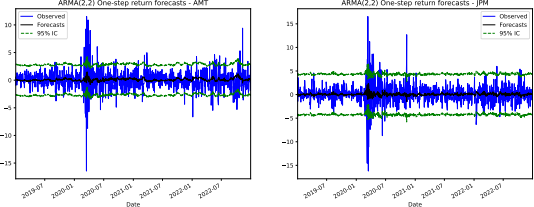
(3 marks)

3.3: Write code to produce one-step analytic forecasts, together with 95% confidence interval, for the returns of each stock using respective best-fitted AR(p)-GARCH(p* , q* ) model found in Task 2.3. For each stock, the forecast output is a data frame with 3 columns f, fl and fu corresponding to the

one-step forecasts, 95% CI lower bounds, and 95% CI upper bounds.                 (4 marks)

3.4: Write code to plot a  1-by-2  subplot figure  showing the one-step return forecasts found in Task 3.3 against the true values during the out-of-sample period for both stocks in your sample. Also show the 95% confidence interval of the return forecasts. Your figure should look similar to the following.

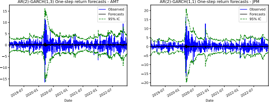
(3 marks)