STA 2023 Written Homework #6
Hello, dear friend, you can consult us at any time if you have any questions, add WeChat: daixieit
STA 2023
Written Homework #6
This assignment is due at 11:59 pm (Beijing time) on the date listed on Moodle but you should work on it throughout the week as you finish each Section (the questions are labeled by Section number). Write all work on separate paper,scan, and submit the assignment to Moodle. Be sure to show all steps for full credit.
1. Section 9.1
In a study of Burger King drive-through orders, it was found that 264 orders were accurate and 54 were not
accurate. For McDonald’s, 329 orders were found to be accurate while 33 were not. Use a 0.05 significance level to test the claim that the Burger King and McDonald’s have the same accuracy rates.
(a) Test the claim using a hypothesis test.
(b) Test the claim by constructing the appropriate confidence interval.
2. Section 9.2
A group of 40 nonsmokers was exposed to second-hand smoke and their cotinine levels (a product of nicotine) had amean of 60.58 ng/mL and a standard deviation of 138.08 ng/mL. Another group of 40 nonsmokers was not
exposed to second-hand smoke and their cotinine levels had a mean of 16.35 ng/mL and a standard deviation of 62.53 ng/mL.
(a) Use a 0.05 significance level to test the claim that nonsmokers exposed to second-hand smoke have a
higher mean cotinine level than nonsmokers not exposed to second-hand smoke.
(b) Construct the appropriate confidence interval for the hypothesis test in part (a)
3. Section 9.3
As part of a national survey, the Department of Health and Human Services obtained self-reported heights (inches) and measured heights (inches) for males aged 12 – 16. Listed below are sample results from the survey. Construct a 99% Confidence Interval estimate of the mean difference between reported heights and measured heights.
Interpret the resulting confidence interval.
|
Reported |
68 |
71 |
63 |
70 |
71 |
60 |
65 |
64 |
54 |
63 |
66 |
72 |
|
Measured |
67.9 |
69.9 |
64.9 |
68.3 |
70.3 |
60.6 |
64.5 |
67.0 |
55.6 |
74.2 |
65.0 |
70.8 |
4 & 5. Section 10.1
For each problem:
(a) Construct a scatterplot and find the value of the linear correlation coefficient, r
(b) Find the P-value and use a significance level of a = 0.05 to determine whether there is sufficient evidence to support aclaim of linear correlation between the two variables.
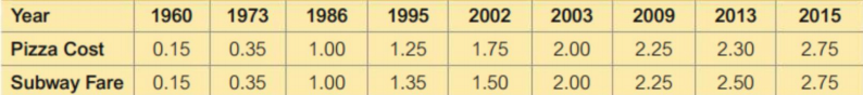
5. The “pizza connection” is the popular idea that the price of a slice of pizza in New York City is always about the
same as a single subway fare. The table below displays the price of a slice of pizza and the subway fare for a sample of years.
6. Listed below are the numbers of registered pleasure boats in Florida (tens of thousands) and the numbers of manatee fatalities from encounters with boats.

6 & 7. Section 10.2
Use the same data as for Questions #4 & 5
For each problem:
(a) Find the regression equation, letting the first variable be the predictor (x) variable.
(b) Find the indicated predicted value by following the prediction procedure summarized on the last slide of the Section 10.2 PowerPoint.
6. Use the pizza costs and subway fares to find the best predicted subway fare, given that the cost of a slice of pizza is $3.00.
7. In a year not included in the sample data, there were 970,000 registered pleasure boats in Florida. Find the best predicted number of manatee fatalities resulting from encounters with boats in that year.
2023-08-07