闪电代写 -代写CS作业_CS代写_Finance代写_Economic代写_Statistics代写_代码代做_IT代写_加急帮助

Hello, dear friend, you can consult us at any time if you have any questions, add WeChat: daixieit

ELEC3114 T2 2023

Introduction

This project involves a two-part task focused on the analysis and control of an inverted pendulum system - a classic problem in control theory. This project encapsulates many of the challenges encountered in real-world control systems. The inverted pendulum is anon-linear and unstable system that demonstrates the effectiveness of various control strategies.

System Modelling

A diagram of the system is provided below, with all reference angles and axes. The definitions and values of the system parameters can be found in Table 1.

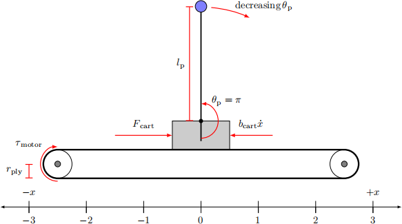
The system above illustrates a cart on a belt driven by a DC motor with a gearbox. That is, the DC motor rotates the pulley on the left by applying a torque, which in turn moves the cart. The pendulum will then move based on the motion of the cart. The recommended equations of motion for the inverted pendulum in the time domain is provided below.

where Fcart is the force applied to the cart in the positive x direction, θp represents the angle between the pendulum and the down-ward position and x represents the displacement of the cart. It is highly recommended that students attempt to derive these equations of motion from first principles (i.e., through the Newton-Euler equations) to identify how the dynamic model is formulated, and how it can be combined with the equations of motion of the DC motor to determine transfer functions between the system outputs and the input voltage. By extension, deriving each equation of motion would also allow students to gain a better understanding on how to convert these to state-space form for more advanced control strategies.

System Parameters

The following constants are provided to align your chosen control strategy with the inverted pendulum simulation within the grader function.

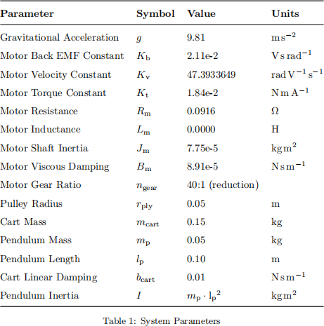
The system parameters can also be obtained in MATLAB using the get parameters() function .

Permitted Assumptions

The following assumptions are permitted in the derivation of the system model and control law(s).

. The timing belt can be regarded as ideal. That is, the timing belt has an efficiency of 100% (ηbelt = 1).

. Model order reduction of the DC motor model is permitted and recommended. How students choose to implement this is up to the student’s discretion.

. Students do not need to consider the height of the cart in their derivations.

Deliverables

Students are expected to produce analytical calculations to support their implementation and simulations in MATLAB. Where the analytical calculations become tedious or complex, students may directly use numerical techniques. However, you must justify why numerical methods were used in these cases. Students must be prepared to justify their design rationale during the Week 11 oral assessment.

Task 1 (6 marks)

Derive a linear model of the inverted pendulum system which takes a single input (voltage, V), and produces two outputs (horizontal displacement, x, pendulum angle, θp ). Produce a simulated time domain response to each of the following inputs,

. no external input (i.e., V = 0 A t e [0, 10]),

. step input (i.e., V = 1 · u(t — 5) A t e [0, 10]).

Students may choose their initial conditions within the following ranges,

. θp (0) = θp-e 干 5deg ,

. θ˙p (0) = 0,

. x(0) = 0,

. ˙(x)(0) = 0,

where θp-e represents the upward equilibrium point. While there are many methods of completing the simulation task1 ., it is highly recommended students use numeric LTI models (i.e., tf, ss) and the associated step, lsim functions.

An auto-test function has been provided for the above method. This will allow students to validate their dynamic models before developing control strategies. The script will validate the given model of the system by comparing the system step response with one given by a solution to the task (to numerical tolerance) and return a RMS percentage error. This is merely to sanity check your linear model, and only serves to ensure students are on the right track in developing a controller for Task 2. Passing the validation script does not yield marks, and marking of this section will be done during the Oral Assessment by checking your analytical calculations and assessing your understanding (similar to lab assessments, where your requirement mark is capped by your understanding mark). The following example shows the use of the validator script.

num_xv = [1 0 0]; den_xv = [1 1 1];

num_thetap = [1 0 0]; den_thetap = [1 1 1];

task1 _validator(tf(num_xv , den_xv), tf(num_thetap , den_thetap));

BONUS Up to 1 marks for the use of Jacobian linearisation in MATLAB. Students must justify their implementation to get the full bonus.

Task 2 (10 marks)

Design a control system which stabilises the inverted pendulum in its upward equilibrium θp = π and the cart at the x = 0 position for a non-π initial swing angle. Once a suitable controller is designed, verify the controller’s operation using the nonlinear model of the system dynamics provided in the grader function. The grader will test the controller’s response with an initial pendulum angle of 180。+ 20。, up to a time of t = 3s. The developed controller(s) must settle within this time. The marks for this section are broken down as follows,

Task 2a (5 marks)

Task 2a solely focuses on the stabilisation of inverted pendulum around the upward equilibrium point θp = π . The control of the cart position is not needed in this task. In other words, the solution is acceptable if the swing is stabilised at any cart position.

. 1 mark for stabilising the inverted pendulum around the upward equilibrium point θp = π within 3s.

. 4 marks from the effectiveness of your control strategy on stabilising the inverted pendulum around the upward equilibrium point θp = π .

Task 2b (5 marks)

Task 2b focuses on the stabilisation of both the inverted pendulum around the upward equilibrium point θp = π and the cart position around x = 0.

. 5 marks from the effectiveness of your control strategy on stabilising the inverted pendulum around the upward equilibrium point θp = π and stabilising the cart position around x = 0.

– 3 marks for just having a control law (i.e., full-state feedback).

– 2 mark for a working implementation of a state observer.

. BONUS 2 marks for a working implementation of a Kalman filter (1 mark) with LQR (1 mark). This also covers the remaining two marks from the state observer section, i.e., 7/5 marks for Task 2b.

Task Grader

Please read the following section carefully. There are several factors which will decide the effectiveness of your control strategy, including the generation of realistic controller outputs, use of state observers, and ultimately, development of a controller which fulfils the control objective.

With the exception of the strategies mentioned in the task restrictions, you may use any control strategy to complete the task. You may even use different control strategies for Task 2a and Task 2b. Most students will initially attempt to use a variation of Proportional-Integral-Derivative (PID) control, but state-feedback control and optimal control strategies can be effective for the both task. The grader function determines two scores based on the following metrics,

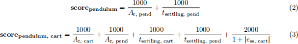
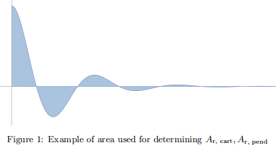
where Ar, cart , Ar, pend represent the area under the cart and pendulum response curves respectively, tsettling, cart ,tsettling, pend represent the settling times, and ess, cart represents the steady state error of the cart.

It should be apparent that the most effective control strategies aim to minimise the parameters above. The final mark for Task 2 will be determined by Equation 4.

where f represents a normalising function determined by the cohort’s performance. The documentation for using the grader is included in the Troubleshooting and Common Questions section below. Your control law should be written as a MATLAB function which follows the following structure,

function u = controller(t , z)

% dt is fixed at 1/200 = 0.005s

% Input Arguments :

% t - Current step time (s) (1x1) .

% z - A vector of doubles representing system state [theta_p;

Dtheta_p; x; Dx] (rad; rads^-1; m; ms^-1) (4x1) .

% Returns :

% u - Controller output/Motor input voltage (1x1) .

u = 0;

end

[t , x , theta_p , score_ 2a , score_ 2b] = task2 _grader(@controller , true);

Constraints

Controllers must not force the motor to be supplied with voltages exceeding the maximum input of 12V. Any controller which violates this constraint will be given a performance score of zero. This means that your controllers must employ strategies to saturate the controller output.

Oral Assessment (5 marks)

Each lab group will be allocated to a 15-minute marking session on Monday, Week 11. Students will be assessed both as a group, as well as individually for this section. During this oral assessment, students will not be allowed access to any resources other than a two-page summary sheet. Use the two pages wisely to write down any necessary notes/details about your implementation for your reference.

Important Notes

Additional Considerations

Task Restrictions

The following control strategies are prohibited in the completion of this task.

. The use of reinforcement learning to update the control law based on performance change over time.

. The use of machine learning to identify arbitrary control laws which minimise a cost function.

. The use of your friend (or internet stranger, generative AI text model) to identify an optimal control law.

The mentioned restrictions do not place a blanket rule on prohibiting machine learning for this con- trol task. Students are encouraged to quantitatively analyse the response to tune and maximise the performance of their system.

Troubleshooting and Common Questions

. My simulation result diverges to infinity. Why?

– There is a good chance your control law responds too slow to the state changes.

. How do I use the grader function?

Syntax:

[t , x , th , score_pend , score_pendcart] = task2 _grader(callable ,

do_plot)

Input Arguments :

callable - A function handle (1x1) .

do_plot - A logical scalar to show response plot (1x1) .

Returns :

t - The simulated time vector (s) .

x - The simulated response of the cart ' s position (m) .

th - The simulated response of the pendulum ' s angle (rad) .

score_pend - Task 2a score .

score_pendcart - Task 2b score .

Example :

[t , x , th , score_pend , score_pendcart] = task2 _grader(@myFunc ,

true);

. I am trying to implement the integral, derivative components, how do I get access to my last states, and preserve a sum across calls of my controller function?

– Make use of persistent (or global) variables. These variables preserve their value from previous scope(s). The following example gives a rough outline of what a derivative implementation would look like. The isempty(prev err) sets the persistent variable on the first function call .

function u = controller_pid(~, z)

persistent prev_err;

if isempty(prev_err)

prev_err = 0;

end

d = kd_t * (err - prev_err) / dt;

last_error = err;

end

Questions and Clarifications

Please direct any clarification questions to the Lab Project Forum channel on teams. However, do not post your source code or solution there. If you have questions about task logistics or the grader, please contact either Dr. Arash Khatamianfar and Barry Feng at the emails below and include ELEC3114 Lab Project in the subject line. We, however, will not debug your programs for you.

. Dr. Arash Khatamianfar - [email protected]

. Barry Feng - [email protected]

Updates to the task

. (17/07/2023) Corrected units and notation for motor back-emf and velocity constants. Updated steady-state error grading criteria for Task 2b to limit the steady-state error score to 2000. Cor- rected md to mcart in Equation 1.

. (07/07/2023) Updated inertia calculation to use point mass at the end of a rod, instead the inertia of the rod itself.

. (04/07/2023) Updated Table 1 to include inertia. Changed labelling of pendulum mass and cart mass to align with get parameters() function .