Hello, dear friend, you can consult us at any time if you have any questions, add WeChat: daixieit

L1025 INTRODUCTION TO STATISTICS

Assessment Period: May/June 2020 (A2)

SECTION A

Answer ALL parts [each part is worth 6 marks, 30 marks in total]

1.

A researcher collects data on annual salaries of senior managers of 12 firms in the hospitality industry. The data is shown in the table below, reported in thousands of pounds.

a. Calculate the mean, median, mode and standard deviation and comment briefly on what these summary statistics tell you about salaries in this industry.

b. Construct a table showing frequencies and relative frequencies of this data. Use class intervals of 0-30, 31-40, 41-50, 51-60 and 61-85. Which interval has the highest relative frequency? [You may find the table layout below useful, edit it as you see fit]

c. Describe how you would represent the relative frequencies on a chart and what it would look like. [For example, explain what type of graph you would use, what it might look like and how you would use it.]

d. The researcher collects more data and, with her new sample from 100 firms, finds the following summary information:

i. What is the probability that a female manager earns between £51,000 and £60,000?

ii. What is the probability that someone earning over £60,000 is a woman?

iii. What is the probability that someone earning £50,000 or less is a man?

e. A larger sample is collected and the researcher calculates a mean salary of £58,000 and a standard deviation of £14,000.

i. What is the probability that a senior manager earns more than £65,000?

ii. What is the probability that a senior manager earns between £42,000 and £70,000?

SECTION B

Answer TWO questions [each worth 35 marks]

2.

a. Explain what is meant by Type 1 and Type 2 errors in the context of hypothesis testing. Which error do we try to minimise when we test hypotheses and why?   [4 marks]

b. A University claims that students spend on average 12 hours a week in the campus Library. Data is collected on a sample of 400 students giving a sample mean and standard deviation of 14 and 4 respectively. Use this data to test the University’s claim, with a significance level of 5%.   [5 marks]

c. Show how your answer to part b would change if the sample size was only 10.   [5 marks]

d. The sample of 400 students consists of 300 undergraduates and 100 postgraduates. Undergraduates spend on average 13 hours a week , with a standard deviation of 6, and postgraduate students spend on average 17 hours a week, with a standard deviation of 3. Test the claim that postgraduates use the Library more than undergraduates.   [8 marks]

e. Among the sample, 100 students live on campus. They spend on average 12 hours a week in the Library, with a standard deviation of 5. Find the 99% Confidence Interval for the population mean.   [5 marks]

f. The survey of students shows that 78% of campus-based students would like the Library to increase its opening hours compared to 82% of off-campus students. Test whether these responses are different. Use a 5% significance level.   [8 marks]   

3.

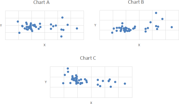
a. The following charts show scatter plots of pairs of variables. Explain which chart shows evidence of:  

i. Positive correlation [2 marks]

ii. Negative correlation [2 marks]

iii. No correlation [2 marks]  

b. A junior economist is examining the relationship between the real price of sugary drinks and consumption. They collect quarterly data for two years, as follows

i. Calculate the Pearson correlation coefficient between price and consumption. Show your working for full marks. What does your answer suggest about the demand curve for sugary drinks? [7 marks]

ii. Test the statistical significance of the correlation coefficient, using a 5% significance level. [7 marks]

c. Using the data in part b), a simple linear regression of the relationship between price and consumption of sugary drinks is estimated and produces the following results:

Consumption  = 7.76 – 0.039 Price

i. Interpret the intercept and slope coefficients   [2 marks]

ii. Predict the amount of sugary drinks consumed when price is £1.28   [2 marks]

iii. Calculate the price elasticity of demand for sugary drinks and interpret your answer. [5 marks] 

iv. Calculate and interpret the goodness of fit, R², for this regression, and use it to test if the model has any explanatory power. .   [6 marks]

4.

You are a junior health economist working for the World Health Organisation and your task is to examine the factors that affect female life expectancy. Using country-level data you estimate the following regression using Ordinary Least Squares:

Life_Expectancy = a + b₁GNP_pc + b₂Births + b₃Civil_War + e

where Life_Expectancy is the number of years a woman born in 2019 may expect to live;

GNP_pc is Gross National Product per capita, measured in $US; Births is the number of births per 10000 women; and Civil_War is a dummy variable which takes values of 1 if the country experienced a civil war in the period 2000-2019, and 0 otherwise.  

You obtain the results shown in the Excel table below. Note that some information has been deliberately omitted.

a. Interpret the coefficients of GNP_pc and Births. [4 marks]

b. Test whether the birth rate has a statistically significant effect on female life expectancy. Use a significance level of 5%. [5 marks]

c. Interpret the P-value for GNP_pc. [5 marks]

d. What is the impact of civil war on female life expectancy? [5 marks]

e. How much of the variation in female life expectancy is explained by the model? [5 marks]

f. Test the null hypothesis that b₁=b₂=b₃=0 [5 marks]

g. Outline briefly how you would attempt to improve this model (no more than 150 words) [6 marks]