Macro-Econometrics Eviews Handout C
Hello, dear friend, you can consult us at any time if you have any questions, add WeChat: daixieit
Macro-Econometrics
Eviews Handout C
This handout provides a brief introduction to estimating and identifying ECM models in Eviews using the Johansen approach. This handout is not meant to be a complete description of this topic. For a more detailed discussion see the appropriate sections in the Eviews manual, available under the Help tab within Eviews.
Consider the example illustrated in the lecture using the simulated variables Y, Z, and W.
The first step (after pre-testing all of your variables) is to estimate a VAR model. You should use a number of tools – LR tests, LM tests, model selection criteria, etc. – to make sure you have the right lag length.
Suppose that you choose a two-lag VAR. The VAR output will look like this:

To conduct the cointegration tests, clicking on View => Cointegration Tests. At this point, Eviews will re-estimate several versions of the model in order to produce the test statistics.
You need to set up various assumptions for Eviews to accomplish this. The first assumption is whether you want to allow constants and/or trends in either the cointegration vector or in the VAR itself.
The default is option #3, which does not allow for a trend in the cointegrating relationship but does allow for a constant in the vector and a possible constant in the VAR itself. For most macro models, this is the correct choice. Log GDP, for example, is often modeled as a random walk with drift.
However, if you have a cointegrating relationship that needs a constant, but you don’t want that constant in the VAR itself (interest rates are a good example, since they are usually modeled as random walks without drift), you can further restrict the ECM by choosing option #2. This option restricts the constant to appear only in the CVs.
Second, you need to enter any exogenous variables – usually not necessary – and you can need to establish the lag length of the VAR, which you have already done in the previous step.
Finally, you can place and test various restrictions on the cointegrating relationship, as discussed in the textbook and the lecture. Initially, you will not want to impose any restrictions on the cointegrating vector.
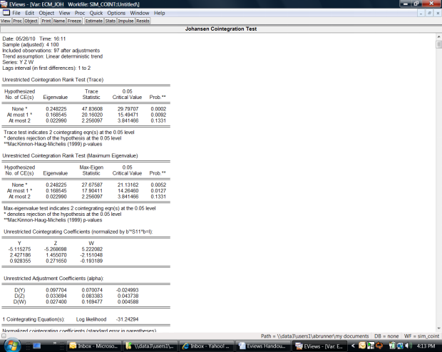
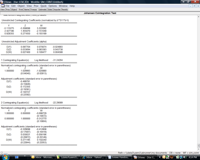
Once you have completed the set-up, click on OK, and Eviews will provide all the output necessary to conduct trace and max tests and analyze the properties of the CV(s) and adjustment coefficients. In this example the output looks like this:
2023-08-02