GEOS1701 ENVIRONMENTAL SYSTEMS, PROCESSES, AND ISSUES (T2 2023)
Hello, dear friend, you can consult us at any time if you have any questions, add WeChat: daixieit
GEOS1701 ENVIRONMENTAL SYSTEMS, PROCESSES, AND ISSUES (T2 2023)
REMOTE SENSING AND ENVIRONMENTAL CHANGE
LAB
Aims and learning outcomes
This lab is designed to test your ability to use some websites that give access to satellite
imagery and image products, focusing on interpreting images and data for identifying environmental change due to bush fires, drought, and floods. You need a basic understanding of how to interpret different false colour composites and NDVI from multispectral satellite imagery, and how to interpret changes in imagery overtime.
Assessment
The concepts explored in this Lab will be assessed through an online quiz.
Materials
As you will use different websites that give access to satellite imagery, you will need a computer connected to the internet and a web browser. You also need to download some kml files from the Moodle page.
Part 1. Bush fires
Firstly, you will look at multispectral satellite imagery from the Sentinel-2 and Landsat satellites, accessed through two websites.

Sentinelhub Playground
https://apps.sentinel-hub.com/sentinel-playground/

You will interpret the environmental change due to bushfires that occurred on the Illawarraescarpment (Maddens Plains) south of Sydney in 2015. You will examine multispectral imagery, and NDVI time series, to assess changes in vegetation cover due to fire and subsequent regrowth.
1.1 False colour composites of bush fires
• Open this website https://apps.sentinel-hub.com/sentinel-playground/
• Turn off the satellite imagery.
• Zoom to Maddens Plains south of Sydney.
• Turn on the Sentinel-2 L1C satellite imagery.
• Change to the “Color Infrared (vegetation)” false colour.
• Change the image date to 14 Jan 2021.
• Change the image date to 1 Jan 2016. You should see the scar of a bushfire in black.
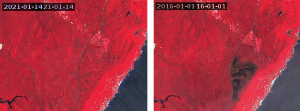
• Zoom in on the area that burnt, and you will see there are some very black patches and some brown patches. Switch to the “Natural color” imagery and see if it is easy to distinguish the fire. Now switchback to the “Color Infrared (vegetation)” false colour imagery and answer the following question.
|
Question 1. Why is the vegetation east of the fire scar a different colour from that to the west of the fire scar? |
• Let’s go back through time to before the fire. If you change the date to 18 Dec 2015, you see the fire, but the image doesn’t cover the whole area. If you go back to the 12 Nov 2015, you can see the fire was yet to occur, but the image contains some cloud and shadow. It is starting to get back to the very early days of Sentinel-2, and there are not many images available.
• Change the Satellite to Landsat 8, then change to the “False color” imagery (this is the same as “Color Infrared (vegetation)” but uses Landsat bands instead of Sentinel-2 bands). Then change the date to 18 Nov 2015.
• Go forward in time by changing the date until you can see the fire scar.
1.2 NDVI of bush fires
• Now you will look at how the vegetation and the fire can be examined using NDVI time-series.
• Open a new browser tohttps://www.sentinel-hub.com/explore/eobrowser/and click “start exploring” .

• Zoom to Maddens Plains south of Sydney.
• In the Discover > Search section uncheck “Sentinel-2” and select “Landsat-8 L2” instead. Then scroll down and hit search.
• Visualise the first image in the search results, then change the image to “False color”.
• Now change the date to 29 Dec 2015 and zoom in on the fire scar.
• Change to the NDVI image.
• Instead of clicking back through past images to see how the NDVI has changed, you can extract atime series of NDVI. Click the polygon button ![]() and then click the upload button
and then click the upload button ![]() . This will bring the following interface, which will let you upload a polygon in different formats.
. This will bring the following interface, which will let you upload a polygon in different formats.
• Load the first of the kml polygons that you can download from Moodle, called maddens_ 1.kml. This is located east of the fire, in the highly photosynthetic vegetation present on the slope of the escarpment.

• Click on the statistics button  to create the NDVI time series.
• The faint envelope around the solid line is the 80% confidence interval (P10-P90), which is greater when the NDVI values of the pixels in the polygon are more variable.
• The noise in the curve is due to cloud in the imagery, which you can remove by
sliding the cloud percentage to zero  Be aware this might remove real data as well as cloud, as clouds are tricky things to identify automatically.
• Move the cloud slider down to 0% and extend the time series back 6 months.
• The NDVI of this vegetation is usually very close to 1, except on 6 Jul, 1 Oct, and 10 Oct 2015. Check the images onhttps://apps.sentinel-hub.com/sentinel-playgroundand answer the following question.
|
Question 2. What is present in the imagery that may have caused NDVI to drop? |
• Remove the polygon with  and load the maddens_2.kml.
• Change the date to 2 March 2016, so that the time series goes past the fire. Make sure the NDVI is selected and then make the time series. Move the cloud slider down to 0% and extend the time series back to 6 months.
• You can see the reduction in NDVI that occurred after the fire, and then the NDVI increases as the vegetation recovers.
|
Question 3. How long did it take for the NDVI to recover to its pre-fire value? |
• Remove the polygon and load the maddens_3.kml polygon and then make the NDVI time series. Move the cloud slider down to 0% and extend the time series back to 6 months. It looks like the NDVI dropped from 0.8 to 0.5 during the fire, but then continued to drop to 0.3 after the fire.
|
Question 4. Did NDVI really continue to drop after the fire, or is something else responsible? |
|
Question 5. Did this area recover to pre-fire levels as quickly as the maddens_2.kml area? What do you think is different about the two areas? |
• Remove the polygon and load the maddens_4.kml and then make the NDVI time series. Move the cloud slider down to 0% and extend the time series back to 6 months. This polygon did not burn, and has maintained an NDVI of around 0.7 throughout the summer of 2015-2016.
Part 2. Drought and flood
In this part of the lab you will look at a drier part of western NSW, where the land is used for grazing native vegetation and some irrigated cropping. The farms around the town of Menindee in western NSW rely on water flowing down the Darling River and filling the Menindee Lakes. In the past the lakes have been very dry, but in the last couple of years they have filled up. To examine changes in water you will use the Sentinelhub Playground and the Digital Earth Australia Maps website.
2.1 False colour composites of drought and flood
• Open a browser and goto https://apps.sentinel-hub.com/sentinel-playground/
• Zoom to the town of Menindee, which is on the Darling River in Western NSW. Change the satellite to Sentinel-2 L1C, and the rendering to the “agriculture” colour scheme. This is based on bands 11 (SWIR), 8 (NIR), and 2 (blue). Dry vegetation is yellow/orange/brown, live vegetation is bright green, and water is blue. This is a nice false colour composite as vegetation stands out as green, and water is blue, which is
what most people expect.
• Zoom out so you can see all the lakes. If you change the date to 7 Jun 2022 you will see a cloud free image, and most of the lakes are full of water, which is blue in this colour scheme. Lots of the land is a shade of brown, orange or yellow, indicating mainly dry vegetation and bare soil. Some of the land around the rivers and lakes is bright green.
|
Question 6. What is the name of the large lake that is dry, on the southern end of the lake system? |
|
Question 7. The lake is divided into paddocks, which are different colours. What has caused some paddocks to be bright green and some light brown? |
• Change the date to 9 Mar 2020, before a flood filled the lakes. You can see some water in the river, but none of it is flowing into the lakes. Now go forward through time and see you the lakes fill up. It is a good idea to move ahead faster by skipping images.
|
Question 8. When does lake Menindee start filling up, and when does it look full? |
• Some of the water in the rivers and lakes is a green colour, rather than blue. Change the image back to the natural colour scheme and see what it looks like. The green water is in fact dirty floodwater laden with sediment.
2.2 DEA Water bodies of drought and flood
• Now you will use the Digital Earth Australia Water bodies dataset to examine the frequency of flooding in these lakes.
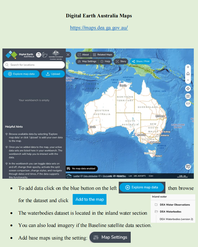
• Open a browser and goto https://maps.dea.ga.gov.au/. Click “explore map data” and add the Digital Earth Australia Waterbodies (version 2) to the map, accessed under the inland water section.
• Zoom to the Menindee Lakes. Note that the southernmost large lake does not have a blue polygon. This means that it has not flooded enough in the last 30 years to be included as a water body.
• Click on Lake Menindee and expand the time series. You will see that in the past there were some long periods when the lake was close to full, but more recently these periods are shorter.
|
Question 9. When was the longest period that Lake Menindee was completely dry? |
• Now click on Lake Tandure, east of Lake Menindee. Click to expand the graph, and now you can compare the time series of the two lakes. Tandure Lake is upstream and receives more regular water than Menindee Lake, which you can clearly see in the time series.
|
Question 10. Why do you think the different lakes receive different amounts of water? |
Part 3. Vegetation clearing and regrowth
The removal of trees to allow land to be used for agriculture is a common practice around the world, and one that can result is many environmental problems such as the loss of habitat and a reduction in biodiversity. The NSW and QLD governments use satellite imagery to detect clearing. In this section of the lab you will need to interpret satellite imagery and NDVI time
series to investigate environmental change in a plantation forest in which trees are periodically planted and harvested. These areas show good examples of how tree clearing looks in imagery, as well as showing areas of trees at different stages of regrowth.
3.1 False colour composites for tree clearing
• Open a web browser and goto https://apps.sentinel-hub.com/sentinel-playground/
• Zoom in on the town of Oberon, New South Wales. It is west of the Blue Mountains and Sydney. You will look at some areas of Blenheim State Forest, which is just northeast of Oberon. If you can’t see the town and forest, turn off the imagery and you will see it on the map.
• Make sure the imagery is set to Sentinel-2 L1C, then change the date to 14 May 2021 and change the rendering to “Color Infrared (vegetation)”.
• You should see several patches of forest, some with stripes and some with a rough, mottled texture.
|
Question 11. What differences in the trees do you think caused the different looking forest? |
|
Question 12. Why do you think the surrounding farmland is a brighter red than the trees in the forest? |
• Go back in time to 24 Feb 2017. You should see many changes in the landscape. The plantation trees are small, and you can clearly see the rows they were planted in. The native trees appear very similar to 2021. Also, in one of the areas that was cleared in 2021, the trees are now visible, and they look like native trees. Also, many of the paddocks in the farmland appear to be bare, which may just be due to the dry summer.
3.2 NDVI for tree clearing
• Now lets look at some NDVI time series of these different forest areas using
https://www.sentinel-hub.com/explore/eobrowser/
• Upload the blenheim_ 1.kml file and the viewer will zoom in on the state forest. Zoom out a bit so you can see the area.
• Now load up some Sentinel-2 imagery, by searching, then visualise a cloud-free images, such as 23 July 2023. Then change the rendering to “False color”.
|
Question 13. What has happened to the forest at and around the polygon? |
• Change the rendering to NDVI, then create a time series plot by clicking the statistics button. Move the cloud slider to 0% and change the scale to 5 years. It might take a while to load the data.
|
Question 14. In what year were the trees cleared? Why did the NDVI not reach zero? |
• Now clear the polygon, change to the False color rendering and load the Blenheim_2.kml file. You should see that this polygon is in the plantation forest.
• Change the date to 4 May 2020, change back to NDVI and create a time series plot by clicking the statistics button. Move the cloud slider to 0% and change the scale to 5 years. Like last time, it might take a while to load the data.
• You should see that the NDVI of this pine forest has a strong seasonal signal. There is also a slight upward trend due to the growing trees.
|
Question 15. In what seasons does NDVI reach maximum and minimum values each year? |
That is the end of the Lab.
You should now have some experience of interpreting false colour multispectral satellite imagery and identifying environmental changes using NDVI and DEA waterbodies.
2023-07-31