This is asummary of topics from the textbook (Nonlinear Dynamics and chaos by steven strogatz) discussed in class.

6.4： Rabbits vs.  sheep

we consider the Lotka-ⅤolteTTa model of competition.  The idea is that there are two species competing for the same food, with limited space.  Let ①(t) be the population of rabbits and g(t) be the population of sheep. The speciic system we consider is

= x (3 - x - 2g),

= g(2 - x - g).

In the  absence  of the  other  species,  each  would  follow  the  logistic  model  (for  example,  if  g  =  O  then = ① (3 - ①), with an unstable ixed point at ①*   = O and a stable ixed point at the carrying capacity ①*  = 3).  However, if there are sheep present, they block the rabbits from getting food, and when there are rabbits present, they block the sheep from getting food.  The magnitudes of the cross terms indicate that the sheep do a better job at blocking the rabbits than vice-versa, and the magnitude of the carrying capacity (in the absence of the other species) show that the rabbits take up less space.  (In a predator-prey model, the sign of the cross term in the predator equation would be positive, whereas here the cross terms are both negative).

Let,s analyze the phase portrait.  The irst step is to ind the ixed points.  By solving = = O we obtain the four ixed points (O, O), (3, O), (O, 2), and (1, 1). The Jacobian is

J(①, g) =  l  3 - 2① - 2g        -2① ) .

(         -g         2 - ① - 2g  )

For (O, O) we have

J(O, O) =  l  3   O  ) .

(  O   2  )

The eigenvalues are λ = 3, 2, therefore we have an unstable node.  The eigenvalue λ = 2 has eigenvector (O, 1)T , and so as t y -钝 typical trajectories will be tangent to the g-axis.

For (3, O) we have

J(3, O) =  l  -3   -6  )

(   O     -1  ) .

The eigenvalues are λ = -3, -1, therefore we have a stable node.  The eigenvalue λ = -1 has eigenvector (3, -1)T . As t y 钝, the typical trajectories will have slope -1/3.

For (O）2) we have

J(O）2) =  l  -1     O   )

(  -2    -2  ) .

The eigenvalues are λ = -1）-2, therefore we have another stable node.  The eigenvalue λ = -1 has eigen- vector (1）-2)T , and so as t 一 钝 typical trajectories will have slope -2/1 = -2.

For (1）1) we have

J(1）1) =  l  -1    -2  )

(  -1    -1  ) .

The determinant is -1, and so we have a saddle.  we can ind the positive eigenvalue λ = -1 +^2 has eigenvector  (^2）-1)T ,  and  so  the  unstable manifold has slope  -^2/2  at  the  saddle,  and  the negative eigenvalue λ = -1 - ^2 has eigenvector (^2）1)T , and so the stable manifold has slope ^2/2 at the saddle. when trying to piece together the overall phase portrait, we notice that g0  = O   =今 g(t) = O for all t. Therefore, we have trajectories lying on the ①-axis. The same holds for the g-axis.

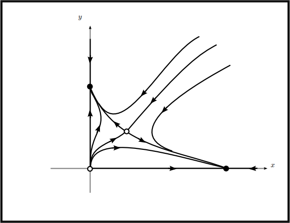
Notice that typical trajectories either approach (3）O) or (O）2).  This means that one of the species will die out, depending on the initial conditions. Moreover, the stable manifold of the saddle separates the basins of attTaction of the two stable nodes.  Therefore the trajectories lying on the stable manifold of the saddle are  called sepaTatTices. The trajectory connecting (O）O) to (1）1) is called a heteToclinic oTbit.

6.5： conservative systems

Linearization is a powerful technique that allows us to conclude whether ixed points in nonlinear systems are stable nodes, stable spirals, unstable nodes, unstable spirals, or saddles (the non-borderline cases). The most important borderline case is a (neutrally stable) center.  Recall the example that showed that when the linearization predicts a center, we cannot conclude whether the ixed point is a center, stable spiral, or unstable spiral in the nonlinear system. our goal for the rest of this chapter is to have some tools that will allow us to ind nonlinear centers.

our deinition of a general conservative system will be motivated by considering a particle on the ①-axis subject to a nonlinear force F (①). Newton,s law F = ma is then

m = F (①).

The force is conseTuatiue because it only depends on position ① — not on velocity or time t.  For such a system, the total energy is the sum of the kinetic energy and the potential energy V (①) which satisies - = F (①).  we claim that the total energy is conserved  (motivating the deinition that this  F (①) is a conservative force). we can calculate

+ V (①)) = m +

= m - F (①)

= (m - F (①))

= O.

Above we used the chain rule, the deinition of V (①), and the oDE. Therefore, the total energy

E := + V (①)

is  constant  in  time.    E  may  be  called  a  conseTued  quantitg  or  fTst  integTal,  we  can  call the  system  a conseTuatiue sgstem. This mechanical system motivates us to deine a conservative system more generally.

Deinition 1. For a system

= f (①, g),

= g(①, g),

a conserved quantity E(①, g) is a real valued continuously diferentiable function that is constant on trajec-

tories : E(.) = O. By the chain rule this is equivalent to

E① f + Egg = O for all (①, g).

In addition, we require E(①, g) to be nonconstant onevery open set (otherwise we could have trivial conserved quantities — for instance E(①, g) = 3 is conserved for every system, and so cannot be useful!).

The existence of a conserved quantity restricts the types of possible ixed points.  (we,ve deined what it means for a ixed point x*  to be  attTacting — all nearby initial conditions approach it as t 喻 … .  A ixed point x*  is  Tepelling if all nearby initial conditions approach it as t 喻 -… . A saddle is neither attracting nor repelling, as there are exceptional initial data (the stable manifold) that approach it as t 喻 … , and exceptional initial data (the unstable manifold) that approach it as t 喻 -… .)

Theorem 1. conseTvative  sgstems   cannot  have  attTacting   (stable  nodes/spiTals)  oT  Tepelling   (unstable nodes/spiTals) f①ed points.

PToof.  (Idea) suppose x*  is attracting.  since all nearby initial conditions approach x*  as t 喻 … , it follows that E(x) = E(x* ) for all nearby x, as E is constant on trajectories and E is a continuous function. However, to be called conservative E must be nontrivial and therefore non-constant on every open set, and we have a contradiction. The same argument works to rule out repelling ixed points.

conservative systems can only have ixed points that are neither attracting nor repelling, which will typically mean they have saddles and centers. More precisely, we have the following.

Theorem  2. consideT a  conseTvative sgstem = f(x)  with f continuouslg  difeTentiable.   suppose x*   is an isolated f①ed point  (f(x* ) = 0 and f(x) 0 foT all otheT neaTbg x) that is a local minimum oT a local ma①imum of the conseTved quantitg E(x) .  Then all tTajectoTies su历cientlg close to x*  aTe  closed oTbits  — that is, x*  is a centeT foT the nonlineaT sgstem.

PToof.  (Idea) since E is constant on trajectories, each nearby trajectory is contained on a contour curve of E. Near local maxima and minima of E, the contours are closed curves.  The only thing that could go wrong is a trajectory does not go all the way around the nearby contour and instead stops at another ixed point. However, we assumed that x*  is an isolated ixed point, so this cannot be the case.

To determine whether a ixed points of the vector ield f is a local minimum or local maximum of the conserved quantity E(①, g), we recall the second derivative test for functions of two variables.

Fact 1. If  E① (①* , g* )  =  Eg (①* , g* )  =  O,  then  (①* , g* )  is  a  critical  point  of  E(①, g).    If,  in  addition, E①① (①* , g* )Egg (①* , g* ) - E①g (①* , g* )2   持 O,  then  (①* , g* ) is either a local minimum or local maximum of E(①, g).

whether it is a local minimum or maximum isn,t important for applying the previous theorem, but it can be done.

Example  1. The  double  well  potential.   consider  a  mass  1 particle on  the  line  with potential energy V (①) = - + . The equation of motion F = ma yields the second-order equation

… dV 3

① =   -      = ① - ① .

d①

The equivalent irst-order system is then

= g,

= ① - ①3 .

The ixed points are (干1, O) and (O, O). The Jacobian is

J(①, g) =  l

(

For the ixed point (O, O) we have

O

1 - 3①2

1  ) .

O  )

J(O, O) =  l  O    1  )

(  1   O  ) ,

which has eigenvalues λ = 干1 with eigenvectors (1, 干1)T .  The origin is then a saddle with stable manifold having slope -1 and unstable manifold having slope 1 at the origin.

For the ixed points (干1, O) we have

J(干1, O) =  l   O

(  -2

1  )

O  ) ,

which has eigenvalues 干^2i, and so the linearization predicts centers.  However, we cannot trust the lin- earization in this case, and showing that these are indeed centers requires considering the conserved energy.

For this type of system arising from Newton,s law, the energy will be

E(①, g) = + V (①),

and so in this case we have

E(①, g) = + - .

You can conirm that E(.)  = E① + Eg = O.   Here,  E① = ①3  - ①2 , Eg   =  g,  and  so we  quickly see that

E① (干1, O) = Eg (干1, O) = O. Furthermore, E①① = 3①2  - 1, E①g = O, Egg  = 1, and so E①① (干1, O)Egg (干1, O) - E①g (干1, O) = 2 持 O, and so each of (干1, O) is either a local minimum or local maximum of E(①, g).  The previous theorem implies then that (干1, O) are centers for the nonlinear system.  The phase portrait is below.

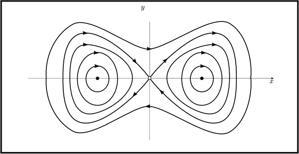
Notice how the unstable manifold of the saddle meets up with the stable manifold — such an orbit that has the same limit as t 一 干钝 is called a homoclinic  oTbit.

6.6： Reversible systems

Many mechanical systems have time-reversal symmetry — the dynamics look the same forward and backward in time. As an example, if you watched a movie of an undamped pendulum, you wouldn,t be able to tell if the movie was playing forward or reverse. More precisely, the equation

m = F (①)

is invaTiant under the symmetry t y -t. This means that if ①(t) is a solution, so is ① (-t).  To see this, we note that although

① (-t) = -(-t)

by the chain rule, the second time derivative

① (-t) = (-t)

is unchanged. Therefore, if ① (t) satisies m = F (①), then so does ① (-t). what does this look like once we switch to a irst-order system？ we have

= g,

= F (①).

since g is the velocity (which was reversed above), this system is invariant under the symmetry t y -t, g y -g.  This means that if (① (t), g(t), is a solution, so is  (① (-t), -g(-t),.  This means that every trajectory has a twin that difers only by g y -g (relection over the g-axis), and t y -t (reversal of the arrow).  This motivates the following deinition.

Deinition 2. The two-dimensional system

= f(①, g),

= g(①, g),

is TeveTsible if it is invariant under the transformation t y -t, g y -g.  Therefore, we need f(①, g) to be odd in g (that is, f(①, -g) = -f(①, g) for all (①, g)), and g(①, g) to be even in g (that is, g(①, -g) = g(①, g) for all (①, g)).

Reversible systems and conservative systems,  though both motivated by Newton,s law  m =  F (①)  are diferent concepts.  There are reversible systems that are not conservative, and conservative systems that are not reversible. However, they have similar properties, and will be another way we can show a nonlinear system has a center.

Theorem  3. suppose  the  sgstem = f(x)  is TeveTsible,  and has  a f从ed point (①* , O)  lging  on the  ① -a从is. If the  lineaTioation pTedicts  a  centeT,  then  it  is  a  centeT foT  the  nonlineaT  sgstem  (that  is,  all  tTajectoTies su历cientlg close to the f从ed point aTe closed cuTves).

PToof.  (Idea) consider a trajectory that starts slightly to the right of the ixed point.  since the linearization predicts a center, we know that the trajectory must intersect a point slightly to the left of the ixed point (we still know the linear center predicts swirling, but we cannot conclude it is a center, stable spiral, or unstable spiral). Then relection over the g-axis and reversal of the arrow gives us the other half of a closed orbit.

Example 2. sketch the phase portrait for the system

= g - g3 ,

= -① - g2 .

we have = O when g = O, 干1.  substituting this into the second equation we obtain three ixed points (O, O), (-1, 1), (-1, -1). The Jacobian is

J (①, g) =  l   O     1 - 3g2   )

(  -1      -2g    ) ,

and so

J (-1, 干1) =  l   O     -1  )

(  -1 士2  ) .

The determinant Δ = -2 for both, and so they are saddles.

For (O, O) we have

J (O, O) =  l   O     1  )

(  -1   O  ) ,

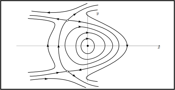
which has eigenvalues λ = 干i, which predicts a center.   Noting that  f (①, g)  = g - g3   is  odd in g, and g(①, g) = -① - g2   is even in g, the system is reversible.  Therefore, the previous theorem applies and the origin is a center for the nonlinear system. The low will be clockwise from inspecting the linearization.

we can use the symmetry across the ①-axis to help with the phase portrait.  For the saddle at ( -1, 1), the eigenvalue λ = -1 +^3 has eigenvector (2, 1 - ^3)T , and so the unstable manifold has negative slope at the saddle.  The eigenvalue λ = -1 - ^3 has eigenvector  (2, 1 +^3) T , and so the stable manifold has positive slope at the saddle.

chapter 7: Limit cycles

A limit cgcle is an isolated closed trajectory.  Isolated means that nearby trajectories are not closed, instead spiraling towards or away the closed orbit.  Therefore, periodic trajectories surrounding a center are not limit cycles, since all trajectories close to a center are closed.

A limit cycle can be stable, unstable, or half-stable. They occur in systems with self-sustaining oscillations, such as the beating of the heart, pacemaker neurons, body temperature, and certain chemical reactions.  They exhibit a preferred period, waveform, and amplitude. The fact that a system has a preferred amplitude for oscillations is an inherently nonlinear phenomenon, since the only periodic solutions for linear systems are centers, where the amplitude is determined from the initial data and not the system itself.

7.1: Examples

Example 3. Many  examples  can  easily be constructed using uncoupled polar equations.   consider  the following system in polar coordinates:

T(.) = T (1 - T2 ),

= 1.

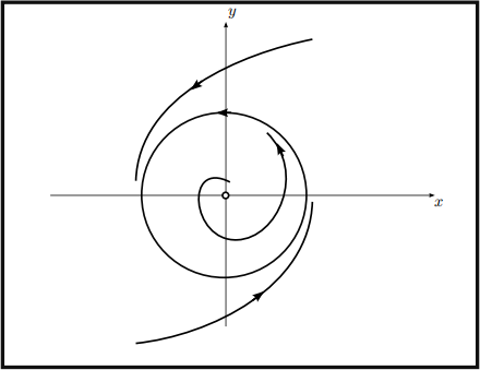
This system is nice because the radial and angular dynamics are uncoupled, so we can analyze them sepa- rately.  The equation means that the angular velocity is equal to one, and so solutions rotate around the origin every 2π units oft. If we consider radial dynamics given by the one-dimensional system T(.) = T (1 - T2 ) for T > O (for us T is a distance and will always be nonnegative), we see there is an unstable ixed point at T = O and a stable ixed point at T = 1.  Then the two dimensional system has the unit circle as a stable limit cycle.

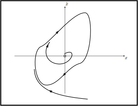
Example 4. The van deT Pol oscillatoT. The van der pol oscillator is given by the second order equation

+ μ(①2  - 1) + ① = O,

where μ 持 O is a parameter.  It describes oscillations in nonlinear circuits in early radios.   consider the damped simple oscillator

+ b + ① = O,

where the damping is a constant b 持 O.  The diference is now the damping factor depends on ① .  when | ① |  持 1, the damping factor is positive and behaves similar to ordinary positive damping.  However, when | ① | < 1 the equation exhibits negative damping. Intuitively, this means large oscillations are damped, while small oscillations are pumped up. It is conceivable then that there is a preferred self-sustained oscillation. In this case the stable limit cycle is not a circle, but a more complicated shape. This is a special case of a Li,enaTd sgstem, and we will have a theorem in section 7.4 guaranteeing the existence of a unique, stable limit cycle for this system.

7.2： Ruling out closed orbits

In sections 6.5 and 6.6, we discussed conservative and reversible systems, and discussed under what conditions they had centers.  Recall a center means there are ininitely many closed orbits, and so we have some criteria that show a system has many closed orbits.  The opposite question would be to show certain systems have no closed orbits — therefore ruling out the possibility of a limit cycle (or of a center).  In this section we will discuss three ways that can sometimes be used to show systems don,t have closed orbits.

Gradient systems

A gradient system is a system of the form

= -ΔV (x),

where V (x) is a scalar function.  That is, the vector ield for the system is the gradient vector ield of a scalar function (up to a minus sign). written out in components, we equivalently have

= -V① (①, g),

= -Vg (①, g).

If this is the case, we call V (x) the potential function for the system (as usual, we assume the vector ield is continuously diferentiable, and so our potential functions will be twice continuously diferentiable). This is the same kind of potential function discussed in 2.7 for one-dimensional systems.

Theorem 4. closed oTbits aTe impossible in gTadient sgstems.

PToof. suppose there is a periodic solution x(t) of period T.  (Recall, built into the deinition of periodic solution is that it is nonconstant — we do not consider equilibrium solutions corresponding to ixed points

as periodic as they are trivial and have nowell deined period).  Then x(o) = x(T), and therefore V（x(o)）= V（x(T)）. on the other hand

V（x(T)）— V（x(o)）= loT V（x(t)）dt.

By the chain rule we have

V（x(T)）— V（x(o)）= loT ΔV（x(t)）. (t) dt）

but since x(t) is a solution to the diferential equation —ΔV = we have

V（x(T)）— V（x(o)）= — loT | (t)| 2 dt < o）

acontradiction. (since x(t) is anonconstant periodic trajectory, 0 for all t since nonconstant trajectories

cannot contain any ixed points). Therefore a gradient system can have no closed orbits.

This is essentially the same argument used in chapter 2 to show that one-dimensional systems cannot have closed orbits — however, all vector ields on the line have potential functions.  For the one-dimensional vector ield = f(①), the potential function essentially the anti-derivative:  — 1 f(①) d① .  However, in more than one dimension, not all vector ields have potential functions. The reason is that for two-dimensions we now are looking for a single scalar function V (①) g) so that

= f(①) g) = — V① )

= g(①) g) = — Vg .

Intuitively, randomly picked f and g will not be compatible.  More precisely, if V is a twice continuously diferentiable function, clairaut,s theorem asserts that V①g = Vg① . If f = — V① and g = — Vg  this means that fg  = g① .  Therefore, a necessary condition for f = (f）g) to have a potential function is that fg  = g① .  It turns out that this is su伍cient in many cases.

Deinition 3. A simply connected region is a region in the plane “without holes”— any closed loop can be continuously contracted to a point without ever leaving the region.

Fact 2. Test to see if a sgstem is a gTadient sgstem — If f(①) g) and g(①) g) are continuously diferentiable on a simply connected set and fg  = g① , then there exists a twice continuously diferentiable function V (①) g) so that f = — V① ) g = — Vg .

Example 5. show that the system

= sing）

= ① cos g

has no closed orbits.

we calculate fg  = cos g, and g从 = cos g.  since f is continuously diferentiable for all of R2  there exists a potential function V.  using technique of exact equations from Math 251 or inding the potential function of a vector ield from Math 23o, we are able to obtain V (①, g) = -① sing.  In any case, closed orbits are impossible in this gradient system.

Lyapunov functions

The key property of gradient systems that excluded the possibility of a periodic solution was the contradiction between a quantity needing to return to the same value while also having to decrease — if x(T) = x(o), then V(x(T))  =  V (V (x(o)), but by integrating along the trajectory we obtain  V(x(T))  < V (x(o)),  a contradiction.  A Lgapunov function satisies a similar property, and the existence of one is a more general condition than the system being a gradient system.

Example 6. show that the system + 3  + ① = o has no closed orbits by considering the total energy

E(①, 2 + ①2 ).

suppose there were a periodic solution of period T.  Then E (① (T), (T)) = E (① (o), (o)).  On the other hand,

E (① (T), (T)) - E (① (o), (o)) = loT E (① (t), (t))dt

= loT + ① dt

= -loT 4 dt 三 o.