6.1.1

we have

 = ① - g）

 = 1 - e从 .

To ind the ixed points, we see that  = O   =院  ① = O, and substituting this into the  equation yields g = O.  Therefore, (O）O) is the only ixed point.

The vertical nullcline is when  = O, and we see it is the line g = ① .  The horizontal nullcline is when  = O, and we see it is the line ① = O (recall the ixed points are when a horizontal nullcline intersects a vertical nullcline).

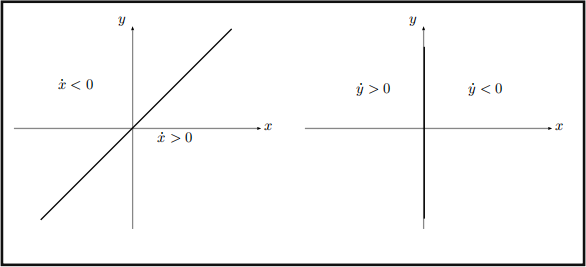
Figure 1:  Along g = ① , we have  = O, and the sign of  is indicated on either side.  similarly along ① = O we have  = O, and the sign of  is indicated on either side.

putting the nullclines together, we obtain the general direction of the vector ield.

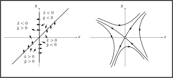
Figure 2: consider the part of the irst quadrant between the g-axis and the line g = ①.  when moving from a point on the g-axis to a point on g = ① , the vector ield must continuously change from pointing left to pointing down, and so you can convince yourself there is a trajectory that goes to the origin as opposed to exiting that region. You can deduce the other parts of what appears to be this saddle,s stable and unstable manifolds similarly.

we might as well use all the tools at our disposal and linearize at the ixed point. we have

J(①, g) =  l    1      -1  )

(  -e从       O   ) ,

and so

J(O, O) =  l   1     -1  ) .

(  -1    O   )

The determinant is Δ = -1 < O and so the ixed point at the origin is a saddle.

6.1.2

we have

 = ① - ①3 ,

 = -g.

This is similar to one of the examples discussed in class — this system is particularly nice as it is decoupled, and we also have some straight line trajectories on the nullclines.  The vertical nullcline, where  = O is just the three lines ① = 千1, O, which are vertical lines and therefore trajectories.  similarly, the horizontal nullcline, where  = O, is just g = O, a horizontal line, and so it is also a trajectory.

since  = -g, we know g will exponentially decay to zero for all trajectories. Thinking of the phase line for  = ① - ①3 , for which ① = 千1 are stable and ① = O is unstable, we can obtain the following starting point for the picture.

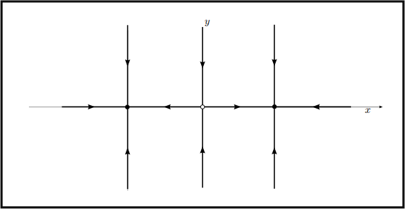
Figure 3: we have straight line trajectories, which forms a nice skeleton for the phase portrait since all we have to do is ill in what happens between these lines — since they are trajectories none of the others can ever cross through them.

It appears then that (干1）O) will be stable nodes and (O）O) will be a saddle. we can conirm by checking the linearization. we have

J (①) g) =  l  1 - 3①2        O   )

(       O         -1  ) ）

and so

J (干1）O) =  l  -2     O   ) .

(   O     -1  )

The eigenvalue -2 corresponds to faster decay as t 一 钝, and so the stable nodes are approached in the direction of the eigenvector for -1, which is (O）1)T , so vertically. At the origin we have

J (O）O) =  l  1     O   ) ）

(  O   -1  )

and so the eigenvalues are 干1, making (O）O) a saddle. The overall phase portrait is below.

Figure 4: we have stable nodes at (干1）O) and a saddle at (O）O).  The stable manifold for the saddle, lying on the g-axis, is the boundary between the basins of attraction for the two stable nodes. The two trajectories making up the stable manifold are called separatrices.

6.1.6

we have

 = ①2 - g）

 = ① - g.

setting  = O we obtain g = ①2 , and substituting this into  = O yields ① - ①2  = O.  Therefore ixed points will have ① = O or ① = 1, and using g = ①2  we ind the two critical points (O）O) and (1）1).

The vertical nullcline, where  = O, is the parabola g = ①2.  The horizontal nullcline, where  = O, is the line g = ①. we then have the following general picture for the vector ield.

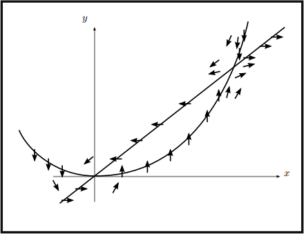
Figure 5: The low is horizontal on g = ① , and vertical on g = ①2 .

using pplane, we can see that the swirling behavior seen near (O , O) is a stable spiral. we can conirm this, along with the saddle at (1, 1) using the linearization. we have

J(①, g) =  l  2①   -1  )

(   1     -1  ) .

For (O, O) we have

J(O, O) =  l  O    -1  )

(  1    -1  ) ,

and so T = -1, Δ = 1, and the eigenvalues are

λ 1 ,2  = -1 干 2(^)1 - 4 = -1 2(干) ^3i .

Therefore (O, O) is a stable spiral, and the swirling is counter-clockwise since

J(O, O) l  1  )      l  O  )

For (1, 1) we have

J(1, 1) =  l  2   -1  )

(  1    -1  ) ,

and so Δ = -1, and so the eigenvalues are real with opposite signs, implying (1 , 1) is a saddle.  The phase portrait is below.

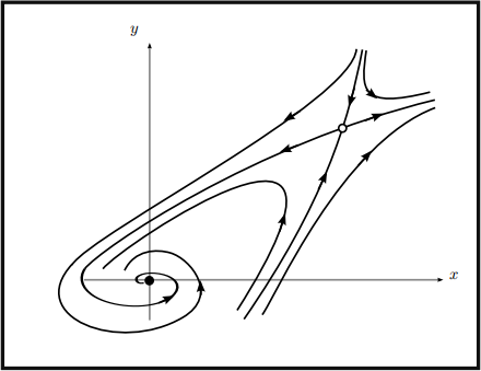
Figure 6: There is a stable spiral at (O, O) and a saddle at (1, 1).

6.3.1

we have

 = ① - g,

 = ①2 - 4.

To ind the ixed points, we see  = O  =今  ① = 干2.  Then substituting into  = O Yields the ixed points (2, 2) and (-2, -2). The Jacobian is

l   1     -1  ) .

(  2①     O   )

For the ixed point (2, 2), we have

J(2, 2) =  l  1   -1  )

( 4     O   ) ,

which has T = 1, Δ = 4. Therefore the eigenvalues are

λ 1 ,2  = 1 干 2(^1) - 16 ,

which are complex with positive real part.  Thus (2 , 2) is an unstable spiral with counterclockwise swirling since J(2, 2)(1, O)T  = (1, 4)T  .

For the ixed point (-2, -2), we have

J(-2, -2) =  l   1    -1  ) ,

(  -4    O   )

which has T = 1）Δ = -4. The eigenvalues are then

λ 1 ,2  =  1 干 ^21 + 16 ）

which will be real and have opposite signs, and so a saddle. The positive eigenvalue has eigenvector (2）1 - ^17)T  and the negative eigenvalue has eigenvector (2）1 +^17)T , and so the stable manifold has positive slope at (-2）-2) and the unstable manifold has negative slope at (-2）-2).

Figure 7: There is a saddle at (-2）-2) and an unstable spiral at (2）2).

6.3.4

we have

 = g + ① - ①3）

 = -g.

setting  = O we obtain g = O, and substituting into  = O we obtain three ixed points, (干1）O)）(O）O). The

Jacobian is

J (①) g) =  l  1 - 3①2        1   ) .

(       O         -1  )

For the ixed points (干1）O) we have

J (干1）O) =  l  -2     1   )

(   O     -1  ) ）

which has eigenvalues λ = -2）-1, and so these are stable nodes.  The slower decaying eigenvalue  λ = -1 has eigenvector (1）1)T  so typical trajectories will approach (干1）O) with slope 1.

For (O）O) we have

J(O）O) =  l  1     1   )

(  O    -1  ) ）

which has eigenvalues λ = 千1, and so it is a saddle.  The eigenvector for λ = 1 is (1）O)T , and the eigenvector for λ = -1 is (1）-2)T .  Therefore the unstable manifold has zero slope at the saddle and the stable manifold has slope -2 at the saddle.  Moreover, if g0  = O, g(t) = O for all t and so we have straight line trajectories on the ①-axis.

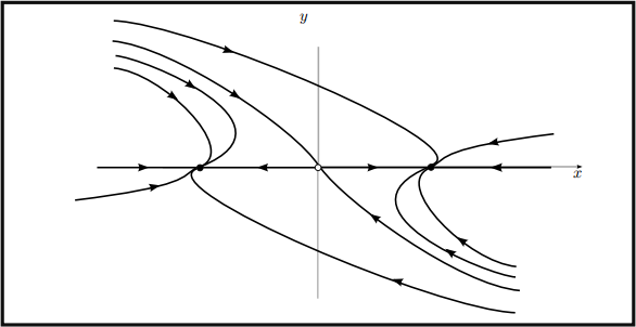
Figure 8: The stable manifold of the saddle at (O）O) is a separatrix — it is the boundary between the basins of attraction for the stable nodes at (千1）O), and it has slope -2 at the saddle.  Typical trajectories approach the stable nodes with slope 1, except for the straight line trajectories along the ①-axis.

6.3.10

(a) The Jacobian is

J(①) g) =  l   g     ①   ) ）

(  2①   -1  )

and we have

J(O）O) =  l  O     O   )

(  O    -1  ) .

The eigenvalues are λ = O）-1 and recall a zero eigenvalue corresponds to a line of ixed points for a linear system.

(b) To show the origin is in fact an isolated ixed point, we just need to solve for all the ixed points and observe that there are no others arbitrarily close to the origin.  = O implies g = ①2 , and then substituting

this into  = O we obtain ①3  = O, and so (O, O) is the  onlg  ixed point for the nonlinear system,  so it is certainly isolated.

(c) The vertical nullclines are when  = O, and so the ① -axis and the g-axis (as the g-axis is vertical we have straight line trajectories on it). The horizontal nullclines are when  = O, and so the parabola g = ①2 .

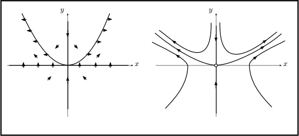
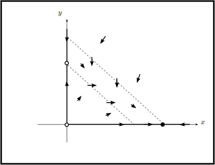
Figure 9:  we still have trajectories approaching the origin along the g-axis, since ①0   = O   =院    ① (t)  = O, g(t) = g0 e-t.  Any initial data in the irst quadrant below g = ①2  will be pushed away, and remain in that region for all future times.

The origin is not repelling due to the trajectories along the g-axis.  It does not seem to be attracting either since initial data above g = O and below g = ①2  will be pushed away.  It seems to be a saddle.

(d)we can use pplane to plot some trajectories.

6.4.1

The ixed points are (O）O), (3）O), and (O）2). The Jacobian is

J(①) g) =  l  3 - 2① - g         -①       ) .

(       -g         2 - ① - 2g  )

For (O）O) we have

J(O）O) =  l  3    O  )

(  O   2  ) ）

which has eigenvalues λ = 3, 2, and so we have an unstable node.  As t 喻 -呐 the eigenmode corresponding to λ = 2 decays more slowly, and so typical trajectories will be tangent to the g-axis since its eigenvector is (O, 1)T .

For (3, O) we have

J(3, O) =  l  -3   -3  )

(   O     -1  ) ,

which has eigenvalues λ = -3, -1, and so a stable node.  As t 喻 呐, the eigenmode corresponding to λ = -1 decays more slowly, and so typical trajectories will have slope -2/3 since its eigenvector is (3, -2)T .

For (O, 2) we have

J(O, 2) =  l   1      O   )

(  -2    -2  ) ,

which has eigenvalues λ = 1, -2, and so a saddle.  The eigenvalue -2 has eigenvector (O, 1)T , and so the stable manifold is vertical at the ixed point.  Moreover, since 从0  = O   =今   从(t) = O for all t, the stable manifold is the g-axis.   The  unstable manifold will have slope  -2/3,  since the eigenvector for λ =  1  is (3, -2)T .

The 从-axis is also invariant, since g0  = O   =今   g(t)  =  O for all t.  There is in fact another straight line trajectory along the line connecting  (O, 2) and  (3, O).   Along  this  line g  =  2 -  从  O, 3)

dg              (2 -  从)(2 - 从 - (2 -  从))

=     =

d从      从(.)           从(3 - 从 - (2 -  从))

= -2/3,

and so trajectories starting on g = 2 -  .

The horizontal nullcline, on which  = O is the 从-axis and the line g = 2 - 从.  The vertical nullcline, on which从(.) = O, is the g-axis and the line g = 3 - 从.