“If have read and I understand the homework set policy in this course.”

in your copy. You should answer this question truthfully before continuing with this home- work set.

1    Pulley contraption attached to a penguin and a trout [20%]

Adapted from Morin, Exercise 3.28, page 76.

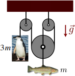
Consider the pulley contraption shown in figure 1.   The larger pulley has two ropes attached to its axle, as shown. One rope is attached to a penguin, via the three pulleys, and the other directly to a trout. The trout has mass m and the penguin has mass 3m.  All the pulleys are frictionless and massless.  Find the accelerations of the penguin and the trout.

Note: if you use software or a calculator to solve thefinal lin- ear system, please indicate which one and which commands you used.

Figure 1: Notations for Q1.

2    F = ma with a F = -bv2 drag force [30%]

Adapted from Morin, Exercise 3.37, page 77.

A particle of mass m is acted upon by a force F (v) = -bv2 .  The particle moves in one dimension and b > 0.

We will do this both analytically and numerically, to compare. 

2.1.  First solve the problem analytically using calculus. Find expressions for the accelera- tion a(t), the velocity v(t) and the position x(t). Take the initial position x(0) = x0 = 0 and an arbitrary initial velocity v(0) = v0 .

2.2.  Next solve the problem numerically, using a time stepping code. Use v(0) = 3.0 m s-1 and b = 0.25 N s2/m2 . You can take m = 1.0 kg.

Do this by modifying the python code called bv2 elpca ofl七 TEpPYATE .oy, which is posted on Quercus.1  Fill in the missing information in the python code for both the analytic expressions and the time stepping scheme. Run the code to make plots for small (like 0.01 s) and large (like 0.5 s) values of d七.  Compare the analytic and numerical plots for various time step sizes.

For this part, make plots with d七 in the titles of the plots and combine them in a single pdf if it isn’t the case already. You do not need to hand in the whole code, the plots will be necessary.

3    Polar coordinates [20%]

This is Morin, Exercise 3.68, page 83.

Consider a particle that feels an angular force only, of the form Fθ  = 3m r˙θ˙ .  Show that r˙ = ± /Ar4 + B, where A and B are constants of integration, determined by the initial con- ditions. Also, show that if the particle starts with θ˙ \= 0 and r˙ > 0, it reaches r 一 o in a finite time.

Note: There is nothing all that physical about this force. It simply makes the F = ma equa- tions solvable.

4   Vibration kinematics [30%]

4.1.  Consider the vibrations x1 = cos(6t) and x2 = cos(7t + π/6). Using Python, plot po-

sition versus time for x1 , x2 , and x = x1 + x2 . What is the beat frequency?  (i.e., the frequency at which minima in the combined signal occur.)

4.2.  Consider the vibrations x1 = 3cos(3t + π/5) and x2 = 4cos(4t + π/8).

4.2.1. What is the expected period for x1+x2?

4.2.2.  Using Python, plot position versus time, velocity versus time, and the phase

space trajectory (i.e., velocity versus position), for x1 , x2 , and x = x1 + x2 .

4.2.3. A solution to Newton’s equation m  = F (x, v) for motion along the x axis is uniquely determined by its initial conditions, which turns out to imply that the phase space trajectory of such a solution should never cross itself. What does this suggest about the combined motion x, given your phase space plot?