Operations Management Re-exam August 2022
Hello, dear friend, you can consult us at any time if you have any questions, add WeChat: daixieit
Operations Management Re-exam August 2022
Solutions
Problem 1
Question 1.1:
In case of moving average with n = 3, there are relevant forecasts from period 4 onward (though it is not entirely wrong to take the average over two periods in period 3, etc.)
The resulting forecasts are:

The forecast in period 4 (F4 ) as a function of demand in period t (Dt ) is:
F4 = (D1 + D2 + D3 ) / 3 = (17 + 16 + 21) / 3 = 18.
The forecast in period 5 is:
F5 = (D2 + D3 + D4 ) / 3 = (16 + 21 + 18) / 3 = 18 1/3 (or 18.3333).
Question 1.2:
The resulting MFE, MAD, and MAPE are:

With formulas:

Computations:
FEt = Dt – Ft, i.e. the forecast error equals demand in the period minus the forecast.
ADt = |FEt | for all t = 4, …, 13 (where ‘ |x |’ is the absolute value of x, other notations can be used). APEt = | FEt / Dt | (because demand is positive, you can also use APEt = ADt / Dt ).
The MFE, MAD, and MAPE are the respective averages of these values.
Question 1.3:
In this question, we have to generate forecasts for MA(3), MA(4) and MA(5). The relevant periods are 6 to 13. For these periods, there are sufficiently many observations available for all three variants. So it makes most sense to compare the forecasts over these periods and consider the forecast accuracy, measured as the MFE and the MAD. (It is a somewhat worse choice to compare the performance of MA(3) over periods 4 to 13 with MA(4) over 5 to 13 and MA(5) over 6 to 13. It is harder to argue for this.) The forecasts and accuracy measures are:
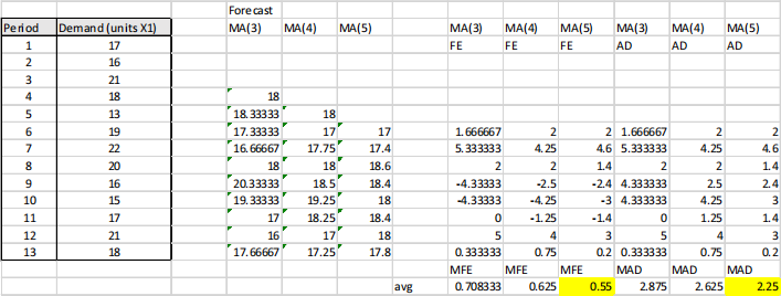
MA(5) scores lowest on both the MFE and the MAD, so it has the lowest bias and the lowest deviation among the alternatives. This method is preferred.
(If you do not select periods 6 to 13 for the comparison, the comparison is somewhat muddied, and you have to make a trade-off between MFE and MAD).
Why? If the best n is large, it is best to consider fluctuations in the data as random (as ‘noise’) to a high degree, rather than as a signal.
Question 1.4:
a) A tracking signal is a measurement that is updated in every period. It is used to check whether the forecast and the observations are sufficiently close to each other. If its value is between -4 and +4, it is. If the value is going outside these bounds, the forecast is straying far from the observations and becomes biased: either too high or too low.
b) In the periods 14 and 15, we compute the following:

Here, the forecast is determined with MA(5). The FE and AD are as previously. Total FE in period 14 equals FE14 , and in period 15 it is FE14 + FE15 . The total AD is computed in a similar way, and MAD(t) = Total AD / number of periods (column ‘Periods). You may also use an average-formula to compute MAD(t), where you fix the first element in the function, so ‘=AVERAGE(x$3:x3)’, and draw it down.
The tracking signal value is 1.68, which is within the prescribed bandwidth.
Question 1.5:
a) The four choices are engineer to order, make to order, assemble to order, make to stock. In this situation, we can observe late customisation in the production process. The best choice is assemble to order (ATO), because this is the form in which the last part of the production process is customised, as is the case here. Make to order is less appropriate, as much of the production of X1, X2, and X3 takes place before a demand order comes in.
b) It is better to use the joint forecasts. The motivation in the textbook is in one of the forecast principles: ‘aggregate forecasts are always better’ (BH p. 278). The reason is that variations in larger populations tend to be smaller than the sum of the variations within their subpopulations, as is stated in the square root law.
Problem 2
Question 2.1:
First-come-first-served rule: As jobs have arrived to the processing centre in the same order that they appear in Table 2.1, they should be processed in the same order according to the FCFS rule. Calculations are done in Excel and screenshots of formulas used for calculations and numerical results are presented below.
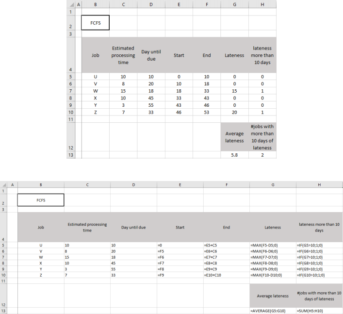
Let STi , ETi , EPTi, and DUDi denote start time, end time, estimated processing time and days until due of job i, respectively.
To make the calculations, we start from the first job – job U. The STU is set to 0. Given the start time, the end time can simply be calculated as the sum of the start time and the estimated processing time. For job U, ETU = STU + EPTU = 0 + 10 = 10. The start time of the next job, i.e. job V, is the end time of the previous job, i.e. job U. For job V, STV = ETU = 10. As we did for job U, the end time of job V can be calculated as ETV = STV + EPTV = 10 + 8 = 18. The same logic holds for the rest of the jobs. See columns E and F for more details.
If the end time of a job is less than or equal to days until due, then the job is not late, i.e. the lateness is equal to zero. However, if the end time exceeds days until due, then the lateness can be calculated as the difference between these two values. To capture both cases, we use Excel MAX() function and compare the difference between end time and day until due with zero. See column G for more details. To indicate if a job is late for more than 10 days, we use Excel IF() function and pass 1 if the lateness is greater than 10 and 0 otherwise. See column H for more details.
Calculating the average lateness and the number of jobs with more than 10 days of lateness is straightforward as shown in G13 and H13, respectively. For the FCFS rule, the average lateness is 5.8 days and 2 jobs experience a lateness longer than 10 days.
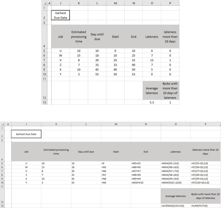
Earliest Due Date rule: According to the earliest due date rule, the jobs should be processed in the order of the days they have until their due dates. Rearranging the jobs based on the days until due date, we get the following sequence: U, W, V, Z, X, Y. The calculations are the same as we did for the FCFS rule. Numerical results and formulas are presented below.
For the earliest due date rule, the average lateness is 5.3 days and only 1 job will be delayed for more than 10 days.
Question 2.2:
Both the average lateness and the number of jobs with more than 10 days of lateness are smaller employing the Earliest Due Date rule compared to the FCFS rule. Therefore, based on these two criteria, the Earliest Due Date rule is recommended.
Question 2.3:
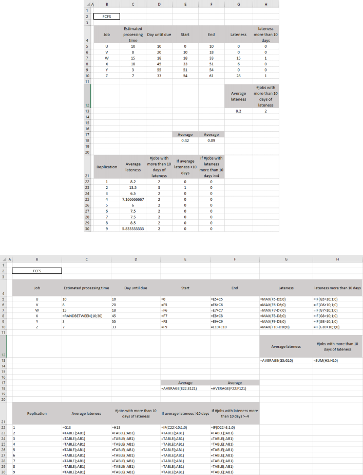
Calculations for the FCFS rule are done in Question 2.1. The only difference here is the estimated processing time of job X which is uniformly distributed in this case. To draw samples from this distribution we can use “RANDBETWEEN(10;30)” assuming a discrete distribution. As it is not clearly specified in the assignment, one can also consider a continuous distribution and use “10+RAND()*(30-10)” in Excel.
For each realization of processing time duration, we calculate the average lateness and the number of jobs with more than 10 days of lateness. Based on these values, one can determine if the average lateness is greater than 10 days and if the number of jobs with a delay of more than 10 exceeds 3. The screenshots of numerical results and formulas are presented below.
The bottom part of the screenshots show the DataTable and the first 9 runs of the simulation model (a total of 100 runs is used here). The DataTable consists of 5 columns. Column B is for replication number. Columns C and D are for the average lateness and the number of jobs with more than 10 days of lateness and the values are directly taken from G13 and H13. In column E, an IF() function is used to indicate if the average lateness exceeds 10 days. In column F, an IF() function is used to indicate if the number of jobs with more than 10 days of lateness exceeds 3. The averages of the columns E and F of the DataTable can be used to estimate the probabilities stated in Question 2.3.
Based on the results shown below,
• the estimated probability of the average lateness exceeding 10 days is 42%, and
• the estimated probability that at least 4 jobs finish with a delay of more than 10 days is 9%.
Question 2.4:
Based on the results in Question 2.3, the requirement is not met as the estimated probability of the average lateness not exceeding 10 days is about 58% (= 100% - 42%) which is much less than 95%.
Problem 3
Question 3.1:
The EOQs of items A and B are respectively

and
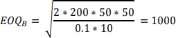
The order size of item A has a duration of 160/40 = 4 weeks, while the order size of item B has a duration of 1000/50 = 20 weeks.
Question 3.2:
a)
If we consider item A in isolation, the optimal review period is 4. Thus, total costs (order and holding costs) of item A are higher for any review period below 4 and increasing again for any review period above 4.
Likewise, if we consider item B in isolation, the optimal review period is 20, and total costs of item B are higher for any review period below 20 and increasing for any review period above 20.
Therefore, the total cost function is decreasing for any review period below 4 and increasing for any review period above 20. This implies that the optimal review period is between 4 and 20.
b)
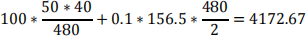
Using Ronny’s proposal, the common review period is (4+20)/2 = 12 weeks. This means the order size of item A will be 40*12 = 480. This gives total annual order and holding costs:
The order size of item B will be 50*12 = 600 giving total annual order and holding costs:

The total annual costs will then be 4172.67 + 1133.33 = 5306.
Question 3.3:
Taking the derivative of the cost function gives
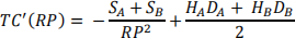
Setting this derivative to zero and isolating RP, gives the square-root formula:
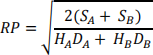
When putting numbers in, we get RP = 0.1332 years. Measured in weeks, this gives RP = 50 * 0.1332 = 6.66. It probably makes most practical sense to let RP be an integer (though in principle there is nothing wrong in using a decimal-valued RP), so let us round it to RP = 7 weeks. This means that the order size of item A should be 40*7 = 280, giving annual costs of

The order size of item B is 50*7 = 350 giving total annual order and holding costs:

The total annual costs become 2905.29 + 1603.57 = 4508.86.
The CEO’s proposal is better. The reason that Ronny calls it “overkill” is probably because he has learned that the cost functions (when doing this sort of EOQ analysis) are in general “flat” . That is, you can deviate quite much from the optimal solution without being penalised very much cost-wise. However, here Ronny deviates quite much from the optimal solution (from 7 to 12). Furthermore, we add two “flat” functions together meaning the total cost function is less “flat”, thereby making it cost more to deviate from the optimal solution.
2023-07-16