闪电代写 -代写CS作业_CS代写_Finance代写_Economic代写_Statistics代写_代码代做_IT代写_加急帮助

Hello, dear friend, you can consult us at any time if you have any questions, add WeChat: daixieit

ECOM055 – Risk Management For Banking

Problem Set 3

Based on Book Chapter 7

L-questions are questions about the lecture and extra materials, H(ull)-questions are question from the book.

L7.1 Use the following excel functions to answer the following questions:

NORM.DIST(x,mean,standard_dev,cumulative)

L7. 1.a What is the cumulative probability of observing Pr(X<Z), if the mean = 0.02, standard deviation = 0.2 and Z = -0.12?

L7. 1.a What is the value of Z for which Pr(X<Z) = 0.01, if the mean = 0.02, standard deviation = 0.2?

L7. 1.a

=NORM.DIST(-0. 12;0.02;0.2;TRUE) = 0.241963652

L7. 1.a

=NORM.INV(0.01;0.02;0.2) = -0.445269575

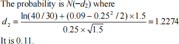
H7.10.

A stockprice has an expected return of 9% and a volatility of 25%. It is currently $40. What is the probability that it will be less than $30 in 18 months?

H7.11.

An investor owns 10,000 shares of a particular stock. The current market price is $80. What is the “worst case” value ofthe portfolio in six months? For the purposes ofthis question, define the worst case value of the portfolio as the value which is such that there is only a 1% chance of the actual value being lower. Assume that the expected return and volatility of the stockprice are 8% and 20%, respectively.

From equation (7.5), the “worst case” stock price is

80exp[(0.08 - 0.22 /2)´0.5+N-1 (0.01)´0.2´ ] = 59.33

The worst case value of the portfolio is therefore $593,300.

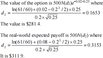
H7.12.

A binary option pays off $500 if a stockprice is greater than $60 in three months. The current stockprice is $61 and its volatility is 20%. The risk-free rate is 2% and the expected return on the stock is 8%. What is the value of the option? What is the real- world expectedpayoff?

L7.2 Monte Carlo Simulations

Estimate the current price of a European call option with a strike price 90 and time to maturity of 1 (year) using a Monte Carlo Simulation. The current stock price is 100, the stock volatility is 0.3 and the risk-free rate is 0.02.

L7.2.a Is this option in, at or out of the money?

Answer:

In the money

L7.2.b Use the Python code from the lecture and the following formula to simulate the stock price at time T (1000 simulations)

S0 is the stock price at time 0, r is the risk-free rate, is the standard deviation, T is the

time to maturity, W is the Brownian motion.

Code:

import numpy as np

import pandas as pd

# Define parameters

risk_free_rate = 0.02

volatility = 0.3

T = 1

num_simulations = 1000

current_stock_price = 100

strike_price = 90

# Generate random draws from standard normal distribution

random_draws = np.random.standard_normal(num_simulations)

# Calculate simulated stock prices

stock_prices = current_stock_price * np.exp((risk_free_rate - 0.5 * volatility**2) * T + volatility * np.sqrt(T) * random_draws)

# Create DataFrame

df = pd.DataFrame({'Random Draw': random_draws, 'Simulated Stock Price': stock_prices})

# Calculate the payoff of the call option

payoff = np.maximum(stock_prices - strike_price, 0)

df['payoff'] = payoff

L7.2.c. Calculate the value of the stock option at the expiration data using the formula C = max(0, S – K). What is the average value of the simulations at time T? What is the present value?

Code

# Calculate the present value of the option

present_value = payoff * np.exp(-risk_free_rate * T)

# Calculate the option price using continuous compounding

option_price = np.mean(present_value)

print("Monte Carlo Option Price:", option_price)

Monte Carlo Option Price: 17.996390810808354

L7.2.d. Compare your estimated value with the value of the option using the Black Scholes option pricing formula. How big is the difference? How big is the difference if you increase the number of simulations to 10.000?

Answer

#BS price

from scipy.stats import norm

# Calculate d1 and d2

d1 = (np.log(current_stock_price / (np.exp(-risk_free_rate * T) * strike_price)) / (volatility * np.sqrt(T)) ) + 0.5 * (volatility * np.sqrt(T))

d2 = d1 - volatility * np.sqrt(T)

# Calculate the option price using the Black-Scholes formula

bs_option_price = current_stock_price * norm.cdf(d1) - strike_price * np.exp(- risk_free_rate * T) * norm.cdf(d2)

# Print the option price

print("BS Option Price:", bs_option_price)

BS Option Price: 18.06906225744624

10.000 simulations