Operations Management Re-exam August 2021
Hello, dear friend, you can consult us at any time if you have any questions, add WeChat: daixieit
Operations Management Re-exam August 2021
Solutions
Problem 1
Question 1.1:
a) The four performance dimensions are cost, flexibility, time, and quality.
b) Time is a very important one. Delays in the deliveries of goods make that TBC may not be able to meet its time commitments, which affects its delivery reliability.
Flexibility can also be affected. If important components are not delivered, then it may not be possible to deliver unexpected quantities or variations of the product.
Quality and cost can also be argued, but in specific cases (e.g., perishable products, cost of expensive replacements to the missing components).
Question 1.2:
a) Portfolio analysis belongs to step 3 of the six-step procurement process, development of a sourcing strategy. We determine the risk and value profile of a product and determine how the supply should be managed in the longer term. For example, should we go for partnership with a supplier, should we automate purchases, should we go for financial benefits?
b) Supply uncertainty is the suggested goal of your sourcing strategy in case of a bottleneck product, i.e., a product with low value but high supply risk. It means that it is important to ensure that supply is there, for example, by having a sufficient supply base or by having extra inventory (rather than trying to obtain products as cheaply as possible, for example).
Question 1.3:
Multiple sourcing refers to the use of multiple, more than one, suppliers. According to B&H Table 7.11, this policy has several advantages compare to the alternative of single sourcing. The most relevant advantage is reduced risk. In that sense, multiple sourcing is better: if a supplier or its supply line is disrupted, we can easily switch to another. (A disadvantage may be that less loyalty is built up, and that a supplier may not work towards a solution when supply is disrupted. But you might be able to use the other suppliers.)
Question 1.4:
Given a projected demand, a TCA compares the cost per unit of making (internally) versus buying (externally). It does so by taking the direct cost (related to the number of products), and the indirect costs, divided by demand, for both options.
Demand = 1mln units
Make (internal)
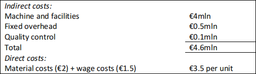
Total per unit: Indirect cost/demand + direct costs = €4.6mln/1mln + €3.5 = €8.10.
Buy (external)

Total per unit: Indirect cost/demand + direct costs = €0.3mln/1mln + €5 = €5.30.
Recommendation: Based on the TCA, buying is clearly cheaper: €5.30 versus €8.10.
Question 1.5:
There are some examples of insourcing in the literature:
Related to CSR, and to the additional file in the syllabus on responsible supply: a company can ensure better that responsible standards are followed in its own company than at a distant supplier. The concrete example is with Mattel, who insourced the monitoring of its own suppliers, so that it could be done according to its own standards. (A similar answer applies to Nestle, who insourcing purchasing of coffee, from middleman, so that it can set the standards and the
Other examples are possible as well, but the answer should have two components. 1) It should be concrete. If the answer starts with ‘Companies…’, it’s usually a generic statement, rather than a concrete one. 2) It should explain how control is taken back, and thereby define what is meant by control. That can be on the standards followed, on the quality of components, on the speed with which items or services can be obtained, etc.
Question 1.6:
a) For each supplier i, we compute its score Pi = ∑j(3)=1 wj sij , where j denotes the criterion (1 = Price, etc.), wj the importance weight of j, and sij the score of i on criterion j. In order to explain this: the columns A,…,D are the j’s, the rows Price,…,Fin. Stability are the i’s, and the numbers under A,…,D
are the scores of the suppliers on the criteria.
The results are as follows:

The computation in Excel for supplier A would be: ‘=SUMPRODUCT(C5:C7;$G5:$G7) ‘, which can be extended to the other suppliers by drawing the formula to the right.
The recommendation is generally to take the supplier with the highest score, which is supplier B (one can observe that the difference with D is small, so this recommendation is not clear-cut).
b) This question tries to probe into the insight into the weighted point evaluation method. The best match is obtained if a supplier scores high on a criterion that also has a high weight in the evaluation (i.e., high piroity). D scores best of all suppliers on criterion ‘Fin. Stability’ . By increasing the weight of this score, we can ensure that D becomes the recommended preferred supplier.
One correct way to do this is to set the weight 1 for this criterion and 0 for the others. D obtains the highest score. It is important to show the results, i.e., that D obtains the highest score for this weight scale.
Another correct approach is to compute a break-even weight for the weight of Fin. Stability, and argue for which increases D is best. This is not strictly necessary, but answers the question well. (The break-even would be attained if we increase the weight of Fin. Stab. to 0.3 and keep all others the same. Now the weights don’t sum to 1 but to 1.05, but one can normalize this by dividing all the weights by 1.05.
Why could such an assessment be relevant? This is an insight question. The scores of the criteria are not easy to determine: it depends on what you prioritize, which may not be so clear. Therefore, you can check whether a minor change in weights leads to a different choice of supplier, i.e., is your choice sensitive to small changes in criteria weights?
(The answer “To initiate negotiations with D” is not accurate. If you negotiate with D, you could try to get a better price. The better price would change the supplier’s score on the performance dimension, rather than the weight).
Problem 2
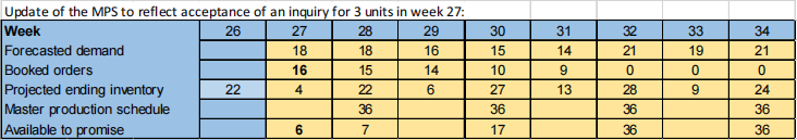
Question 2.1:
The master production schedule for VacZ becomes:
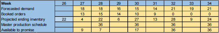
Forecasted demand (F) and Booked orders (OB) consists of the data from the problem text. Projected ending inventory in week t (EIt) is calculated by using formula (12.1). For example, the ending inventory in week 28 is obtained as: EI28 = EI27 + MPS28 – max(F28, OB28 ) = 4 + 36 – 18 = 22.
Available to promise (ATP) is calculated by using formulas (12.2) and (12.3). For example, the available to promise in week 27 (the first period here) is obtained from (12.2) as: ATP27 = EI26 + MPS27 – sum(OBt), for t = 27, or 9 = 22 + 0 – 13. The available to promise in week 28 is obtained from (12.3) as: ATP28 = MPS28 – sum(OBt) for t = 28, 29, or 7 = 36 – (15 + 14).
The productions lots, each consisting of 36 units, are placed in those weeks where the ending inventories would become negative if no production took place.
Question 2.2:
a) Inquiry no. 1 for 13 units in week 28 is accepted because the ATPs in weeks 27 and 28 (16 units) are sufficiently large to cover it:
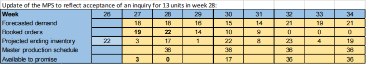
In week 28, 7 units are transferred from ATP to OB and, in week 27, the remaining 6 units requested are transferred in the same way. Note that transferring instead 9 units in week 27 and 4 units in week 28 would be more restrictive as that would leave no ATPs left in week 27 (making the transfers in this way is considered as a small mistake as it would lead to inquiry no. 3 being rejected).
Inquiry no. 2 for 8 units in week 29 is rejected because now there are only 3 units of ATP available for week 29.
Inquiry no. 3 for 3 units in week 27 is also accepted because there are 3 units of ATP available for week 27:

The requested 3 units in week 27 are transferred from ATP to OB. The negative ending inventory in week 29
results because forecasted demand exceeds booked orders. This is not a real problem as long as no more orders are booked for this week.
Inquiry no. 4 for 8 units in week 34 is accepted as there are plenty of units of ATP available for week 34:
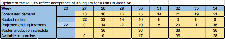
In week 34, 8 units are transferred from ATP to OB.
b) Inquiry no. 3 is accepted because there are more than 3 units of ATP available in week 27:
Transfers from ATP to OB are made in the same way as in part a) and will not be mentioned here. Inquiry no. 1 is accepted because there are 13 units of ATP in weeks 27 and 28:
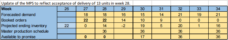
First, 7 units are transferred from ATP to OB in week 28, and then the remaining 6 units are transferred in week 27. Again, the negative ending inventory in week 29 results because forecasted demand exceeds booked orders.
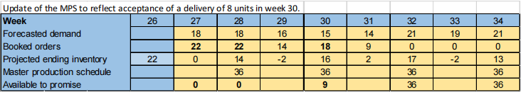
Inquiry no. 2 is accepted because 8 units can be delivered in week 30 (only one week late):
Inquiry no. 4 is also accepted as this can easily be booked without any delays:

c) Under the rule in part a), only three requests are accepted for a total of 24 (13 + 3 + 8) units. Under the rule in part b), all requests are accepted for a total of 32 units.
In part b), one customer experiences a minor delay of one week, whereas in part a) this customer’s request is completely rejected. Therefore, all customers should be happy with the rule in part b). For the company, the scenario in part b) is an advantage because they are able to sell more units and thereby retain happy customers.
Question 2.3:
From the MPS for VacZ, we obtain the information shown below. Note that information about production lead time is missing in the text, and therefore an assumption must be made. Here it is assumed that the lead time is one week.

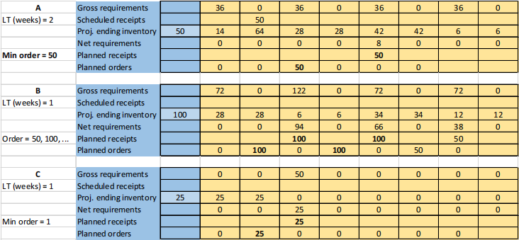
We must set up the MRP for ingredient A before that for ingredient B, because we must know the requirements for A before we can determine requirements for B:

Gross requirements come directly from the Start assembly of VacZ. Projected ending inventories and Net requirements are obtained by using formulas (12.5) and (12.4), respectively. The positive net requirement in week 36 triggers a planned receipt of 200 units (min. order size). Planned order releases are obtained by taking the 2-week lead time into consideration.
Next, we set up the MRP for ingredient B:

Here, Gross requirements come from two sources: the start assemblies for VacZ (two units for each VacZ) and the planned orders for ingredient A. For example, the gross requirements in week 29 are obtained as: 272 = 2 times 36 + 200.
Planned receipts are determined as the smallest multiple of 50 units that is sufficient to meet the net requirement for the week in question.
Finally, we set up the MRP for ingredient C:
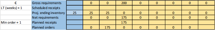
Here, Gross requirements come directly from the planned order releases for ingredient A. Planned receipts are all equal to the net requirements in each week.
Question 2.4:
a) Changes occur in the MRPs for all three ingredients:
A planned receipt of 50 units of ingredient A is now sufficient in week 36 (as opposed to the original 200 units). This change propagates to the planned receipts for ingredients B and C, which become considerably smaller (only 100 units of ingredient B in week 29 instead of 250 units and only 25 units of ingredient C in week 29 instead of 175 units).
b) It is well known in MRP systems that large minimum order sizes sometimes have adverse consequences. As we can see in the answer to part a), planned order releases in an MRP at one level of the BOM propagate to MRPs at lower levels of the BOM. This means that any change to a large order at an upper level may have dramatic effects at the lower levels.
We see that reducing an order for ingredient A, actually has quite large effects on the sizes of the order releases for ingredients B and C.
Problem 3
Question 3.1:
While the process is as it should be, n samples, each of size m, are collected. Control charts are created based on these samples. Besides “target values”, the control charts contain lower and upper control limits. After the control charts are created, we continue to take samples. Each sample is plotted in the control chart and it is checked that it falls between the control limits.
Question 3.2:
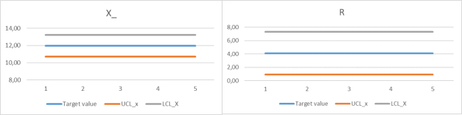
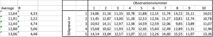
Based on the information in the table, we can determine the average and the range for each sample.
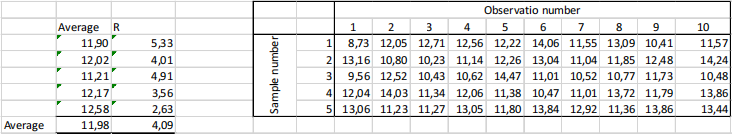
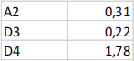
The sample size is 10. Therefore, the relevant values from table 5.4 in the book are
We now use formulas 5.9-5.12 to determine the control limits as
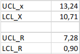
The resulting control charts look like this:
Question 3.3:
For each sample, we again compute the average and the range, and get
We can now plot these into the control charts:
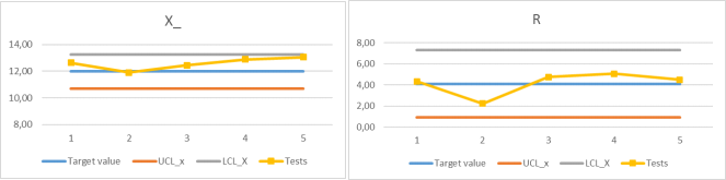
Both the average and the range stay within the control lines so in theory, all is fine. However, the average is repeatedly close to the upper limit, which is a sign that the process needs extra attention.
Question 3.4:
The simulation model can be set up like this, where formulas are shown below.

Note that
• The strength of the raw medicine is simulated by the use of a lookup function based on the distribution provided in the table of the assignment.
• The strength of the finished medicine is simulated by a normal distribution, where the mean is the simulated strength of the raw medicine and the standard deviation is 1.
Question 3.5:
The strength of the finished medicine is now simulated with 200 repetitions in a data table. Based on these simulated numbers, we can determine the average strength, and use
• =COUNTIF( the data table values ;"<"&10.5) to determine the number of portions that are too weak.
• =COUNTIF( the data table values ;">"&13.3) to determine the number of portions that are too strong.
• The remaining portions are useful.
We observe that the average is higher than the one we found in Question 3.2, and the range is significantly higher. This indicates that the production process is not as good as it was when it was first developed. We find that only 64.4% for the portions are useful in the end and 35.8% are discarded. We also notice that even though we use 200 repetitions in the simulation, the numbers are not stable.
2023-07-13