COMP809 – Data Mining and Machine Learning Lab 10 – Neural Network/ MLP
Hello, dear friend, you can consult us at any time if you have any questions, add WeChat: daixieit
COMP809 – Data Mining and Machine Learning
Lab 10 – Neural Network/ MLP
This lab covers implementation related to Multi_Layer Perception (MLP) classifier using the sklearn module. In addition to the implementation of the classifiers, you will learn how to display important curves/graphs using loss/accuracy. This lab provides detailed implementation of the Multi-layer Perceptron (MLP), a supervised learning algorithm, using a real-world dataset. Diabetes is a chronic disease that occurs either when the pancreas does not produce enough insulin or when the body cannot effectively use the insulin it produces. Insulin is a hormone that regulates blood sugar. Hyperglycaemia, or raised blood sugar, is a common effect of uncontrolled diabetes and over time leads to serious damage to many of the body's systems, especially the nerves and blood vessels. The Diabetes dataset used in this lab holds several medical predictor variables and one target variable, Outcome. These data are collected from female patients at least 21 years old of Pima Indian heritage residing near Phoenix, Arizona. More information can be found in UCI Machine Learning Repository. The objective of this lab is to use the MLP model to predict whether or not the patients in the dataset have diabetes or not.
1. Importing libraries
Task 1.1: Import related libraries such as
a. Numpy;
b. train_test_split;
c. accuracy_score;
d. MLPClassifier (from sklearn.neural_network) ;
e. matplotlib.pyplot;
f. pandas.
2. Create a Data Frame
Task 2.1: Read your dataset into a data frame and observe the content of your dataset.
diabetes = pd.read_csv('Diabetes_Data.csv')
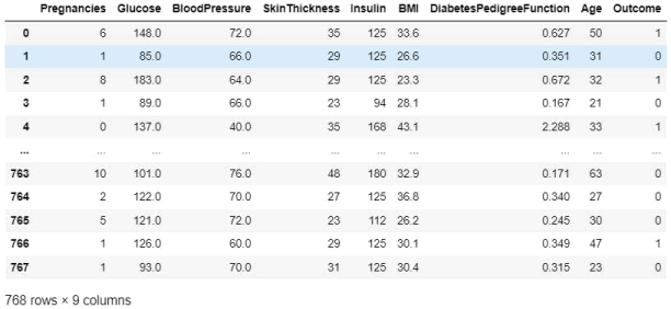
Figure 1: Features presented in the ‘Diabetes_Data’ dataset.
There are 768 instances in the dataset. The dataset holds the following 9 attributes:
1. Number of times pregnant
2. Plasma glucose concentration 2 hours in an oral glucose tolerance test
3. Diastolic blood pressure in mm Hg
4. Triceps skin fold thickness in mm
5. 2-Hour serum insulin in mu U/ml
6. Body mass index measured as weight in kg/(height in m)^2
7. Diabetes pedigree function
8. Age in years
9. Outcome (1:diabetic or 0:healthy) (class)
3. Assign Variables Use the first 8 columns as input/predictors and the last column (Outcome) as output/target.
Task 3.1: Assign predictors (your feature dataset) and target (your class label dataset)
4. Explore the Data Perform initial data exploration through Tasks 4.1 and 4.2.
Task 4.1: Check the class distribution by plotting the count of outcomes by their value. Explain your findings.
Task 4.2: Create a Pearson's heatmap to explore the correlation between the inputs/predictors and the class. Explain your findings.
5. Rescaling the Data Looking at your input data, you will notice that the data in each column have
different ranges. It is recommended to bring all the features to the same scale through rescaling.
Task 5: Rescale your dataset usingsklearn's standardscaler
6. Train and Test Split with Stratification Split your dataset to train (70%) and test sets. The test set holds data to be used for evaluating the model that has been created using the train set. Stratification helps to accommodate the problem of ‘imbalanced’ data. The ‘stratify 'parameter in train_test_split() will ensure that both training and test sets have the same proportions of the class labels.
Task 6: Split your dataset using sklearn’s train_test_split(), and set the stratify parameter to accommodate the problem of ‘imbalanced’ data.
i. features dataset for training
ii. features dataset for testing
iii. class label dataset for training
iv. class label dataset for testing
7. Create the Model and Make Prediction:
Task 7.1 Develop a Multilayer Perceptron (MLP) model for the dataset using SciKit Learn MLPClassifier. Build the model with 200 iterations (chosen arbitrarily) with the solver for weight optimization set to the ‘adam’ version of stochastic gradient descent (it will automatically adapt the learning rate).
• Activation function = 'logistic'
• solver for weight optimization = 'adam'
• learning rate = 0.01
Task 7.2: Fit Model and Make Prediction Use the fit() method to fit the MLP model to the training data for the prediction.
Task 7.3: Adjust the configuration before evaluating models. It is a good idea to review the learning dynamics and tune the model architecture and configuration until we have stable learning dynamics, then look at getting the most out of the model. Obtain the ‘loss_values’ and plot it. Explain your findings and adjust the ‘max_iter’ parameter value accordingly.
8. Evaluate Model Performance
Task 8: At the end of the training, evaluate the model’s performance on the test dataset and provide the model Accuracy, classification report, and score on the training and test sets. Explain your findings.
9. Confusion Matrix
Task 9: Now check the confusion matrix and the score of the predicted values. Visualize the confusion matrix of the predicting values and explain your findings.
10. Robust Model Evaluation Through k-fold Cross-validation Now that we have some idea of the learning dynamics for a simple MLP model on the dataset, we can look at developing a more robust evaluation of model performance on the dataset. The k-fold cross-validation procedure can provide a more reliable estimate of MLP performance, although it can be very slow as ‘k’ models must be fitted and evaluated. This is however not a problem for a small dataset, such as the cancer survival dataset.
Task10: Use theStratifiedKFoldclass and enumerate each fold manually, fit the model, evaluate it, and then report the mean of the evaluation scores at the end of the procedure.
11. Create the Confusion Matrix from k-fold Cross-validation
Two functions, ' generate_confusion_matrix’ and ‘p l ot _ c onf us i on _ m at r i x ’ , are written to generate and plot the confusion matrix from k-fold Cross-validation. Study these two functions to figure out a) which one should be called to obtain the confusion matrix and b) which variables from Task should be passed to that function.
Q1: Provide the confusion matrix (Confusion Matrix from k-fold Cross-validation) and explain the classification model performance.
Q2: Using Q1’s generated confusion matrix, calculate and provide the evaluation metrics including ‘accuracy, precision, recall, and f1-score. Include the calculation formula in your answer and explain your findings. Refer to your lecture notes for calculation steps. You also might find thislink useful.
2023-06-30