Learning outcomes assessed

This coursework will test some concepts of Matlab programming for data analysis, including writing scripts, functions, advanced plotting, manipulating strings and using cell arrays and structure variables.

Instructions

Put your marking ID on your solutions. You can obtain your marking ID by running the command getmarkingid while logged into linux.cim.rhul.ac.uk. Please do not put your name on your solutions. Please make a copy of your solutions before submitting. Your solutions will not be returned together with the feedback. 

You will submit your work electronically by means of the submission script submitCoursework which can be found on linux.cim.rhul.ac.uk. You may resubmit your script any number of times, though only the last submission will be kept. 

The submission will occur on linux.cim.rhul.ac.uk and the protocol is:

For example, assuming the directory with my solutions is assignment1 then I would submit by typing in the following command:

submitCoursework assignment1

and then follow the instructions accordingly. 

The files you submit cannot be overwritten by anyone else, and they cannot be read by any other student. You can, however, overwrite your submission as often as you like, by resubmitting, though only the last version submitted will be kept. Submission after the deadline will be accepted but it will automatically be recorded as being late and is subject to College Regulations on late submissions. Please note that all your submissions will be graded anonymously. 

IMPORTANT: For this assignment you will have to submit:

• A file containing function plotrandstem required for exercise 1.
  
• A file containing function myplots required for exercise 2.
  
• A file containing function mykmeans required for exercise 3.
  
• A file containing script docdistances required for exercise 4.
  
• A file containing script PCAEx5 required for exercise 5.
  
• A file containing function subtractMean required for exercise 5.
  
• A file containing function myPCA required for exercise 5.
  
• A file containing function projectData required for exercise 5.

The following files are provided for the exercises:

• A file pointsEx1.txt required for exercise 1.
  
• A file DataForKmeans.mat required for exercise 3.
• Six files containing text of RedRidingHood.txt, PrincessPea.txt, Cinderella.txt, CAFA1.txt, CAFA2.txt and CAFA3.txt required for exercise 4.
  
• A file pcadata.mat required for exercise 5.
  
• A file pcafaces.mat required for exercise 5.
  
• A file containing a function recoverData.m required for exercise 5.
  
• A file containing a function displayData.m required for exercise 5.

If you will write any other extra function or script as part of your solution for these exercises, you should also submit these. For these extra functions or scripts, you can choose the file name. A zip file containing a template for each of these files is provided on the course page on Moodle. You need to insert your code for each exercise where indicated and submit them. 

All the work you submit should be solely your own work. Coursework submissions are routinely checked for this.

EXERCISE 1 (3 points)

Write a function plotrandstem that will receive two parameters as input: the name of a text file and a number n. The text file to be used as input to plotrandstem is already provided on the Moodle page (file pointsEx1.txt). plotrandstem will read pointsEx1.txt which contains the x and y coordinates for the data points and will create a stem plot using n points chosen at random. The format of every line in the file is the letter ‘x’, a space, the x value, a space, the letter ‘y’, space, and the y value. The number of points drawn will be shown in the plot title. For example, the function call: 

will produce something like the following Figure:
Your function will need to check that the value of n is smaller than the total number of data points in the file, and provide the user with an appropriate error message in case it is bigger.
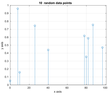
(HINT: you could use fopen followed by fscanf to read the file). 

EXERCISE 2 (4 points)

Write a Matlab function myplots that will received three input arguments:

1. a cell array containing 4 strings taken from the set {sin, cos, tan, sinh, cosh, tanh}

2. a vector of 4 characters specifying a colour taken from the set {k, m, c, r, g, b}

3. a vector of 4 markers taken from the set {+, o, *, x, s, p}.
Your function should produce one figure containing 4 subplots.

Your function should produce one figure containing 4 subplots.
The first subplot will contain the plot of the first mathematical function in the cell array (that is, the first string in the cell array). The second subplot will contain the second one, and so on for all 4 subplots. The title of each subplot should indicate the mathematical function being plotted. 

The mathematical function in subplot i, will appear with colour and marker as specified by the corresponding i entries in the second and third input vectors. All mathematical functions should be plotted in the interval [-2, 2] with a step of 0.3 and a marker should appear at each step. 

Your matlab function should output an error in case the input vectors have length different than 4.

For example, the following call to myplots:
myplots({'sin', 'sinh', 'cos', 'cosh'}, ['b', 'r', 'k', 'g'], ['o', 'x', 's', '*'])
will produce something like this:

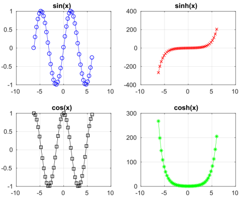
(Hint: the matlab function eval can be useful here.)

EXERCISE 3 (8 points)

In this exercise, you will write a vanilla version of the well-known k-means clustering algorithm for data points in 2 dimensions – this algorithm is part of the Data Analysis course. Briefly, the algorithm partitions a dataset of n points into k disjoint clusters; each cluster is identified by a centroid which changes its position during the learning; each point belongs to the cluster whose centroid is nearest to it. 

The algorithm that you will implement is as follows:

• Step 1: Random initialization of the centroids from the data. Select k points at random from the dataset as initial centroids.

• Step 2: Compute the Euclidean distances between the data points and the centroids. [Hint: use the build-in function pdist2].

• Step 3: Assign each point to the centroid which is closest to it.

• Step 4: Update each of the K centroids by moving it to the mean of all the points which were assigned to it.

• Step 5: Go to Step 2

Stopping criterion: The loop (steps 2 to 5) stops when the position of the centroids does not change between two consecutive iterations.

In this exercise you will write the function mykmeans that receives two inputs:

1) a dataset of n points in 2D (an example is provided in the file DataForKmeans.mat)

2) the number of clusters k.

mykmeans will implement the algorithm described above and will:

1) Return a matrix C of size k x 2, containing the final position of the centroids, one centroid per row.

2) Return a vector V specifying the cluster to which each point belongs. This vector will have n elements, and the ith element will contain an integer in the range [1, k] indicating the cluster to which the ith element belongs (note that V(i) specifies the cluster having C(V(i),:) as its centroid).

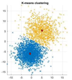
3) Plot a figure showing the different k clusters obtained, in different colours, together with their centroids – make sure the centroids are clearly visible in the figure. For example, using the data provided in the file DataForKmeans.mat, the call to the function: [C, V] = mykmeans(Data, 2);

produced the following figure (here the centroids are drawn as large red diamonds).

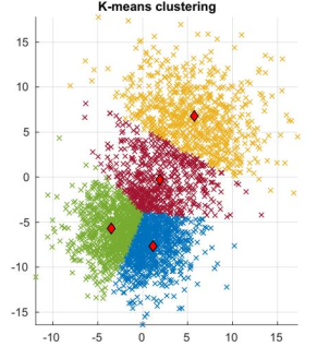
The call to the function:

produced the following figure:

[Warning: the above figures should only be taken as references since every run of k-means is likely to produce different clusterings as the algorithm is affected by local minima].

Finally, note that this exercise is about implementing k-means yourself, so you cannot use the kmeans function available in Matlab.
EXERCISE 4 (10 points)
In this exercise you will write a script called docdistances that will calculate distances between pairs of text documents. These distances will be based on a vanilla version of term frequency–inverse document frequency (tf-idf). Your script will calculate the distances between 6 documents: 3 documents are synopsis of fairy tales (Red riding hood, the Princess and the pea and Cinderella); the other 3 documents are the abstract of papers related to protein function prediction (identified as CAFA1, CAFA2 and CAFA3). You will find these documents on the Moodle page (the files name are: RedRidingHood.txt, PrincessPea.txt, Cinderella.txt, CAFA1.txt, CAFA2.txt, CAFA3.txt).
Your script will:
1. For each document, calculate its tf-idf vector.
The tf-idf vector of a document is a vector whose length is equal to the total number of different terms (words) which are present in the corpus (in this case, the corpus is the entire set of 6 documents). Each term is assigned a specific element of the vector, which is in the same position for the tf-idf vector of every document. For a given document d, the vector element corresponding to term t is calculated as the product of 2 values:
a) Term frequency: the number of times that term t appears in document d
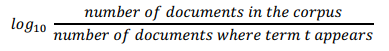
b) Inverse document frequency: the log base 10 of the inverse fraction of the documents that contain the term, i.e.

2. Calculate the cosine distance between every pair of tf-idf vectors representing each document. (This is equal to 1 minus the cosine of the angle between the 2 vectors.)
3. Collect these distances into a 6x6 matrix where the value in the (i,j) element contains the distance between document i and document j. Then make a figure that displays the matrix. Your Figure should look similar to the Figure below (here I have used imagesc and set the colormap to gray).

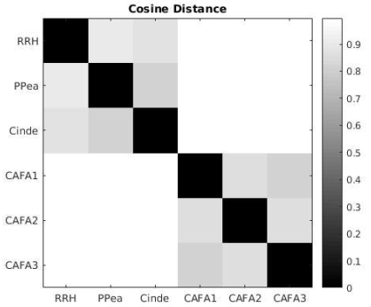
It is interesting to note that the 2 types of documents form 2 clear groups: the synopsis of fairy tales are more similar to each other than they are to scientific papers. Also, the Princess and the pea is more similar to Cinderella than to Red Riding Hood, and this makes sense as the Princess and the pea and Cinderella have many more elements in common …
[HINT: the functions textread and pdist could be useful for exercise 4]

EXERCISE 5

In this exercise you will explore Principal Components Analysis (PCA). The exercise is divided in 2 parts. In the first part, you will work with a small toy dataset of artificial data, developing functions needed for carrying out PCA. In the second part, you will work with a larger dataset of real world data (images of faces of famous people), and you will be able to re-use the functions you wrote for the small toy dataset on a larger scale. Note that this is a good approach to use when implementing algorithms: make sure that they work well on small datasets and then apply them to your real problem. Remember that the implementation for the small dataset needs to be efficient, otherwise its execution time will be very large when applied to the larger dataset. 

For both datasets, you will:
1. Calculate the principal components of your data
2. Project your high dimensional data onto (a smaller space defined by) a few principal components
3. Recover your original high dimensional data by re-projecting back the projected data onto the original space.
Note also that this exercise is about implementing PCA yourself, so you cannot use any of the different functions available in Matlab which implement it (e.g. pca). You will have to calculate the principal components through the eigendecomposition of the covariance matrix of the data (you will need to use the Matlab function eig for the eigendecomposition).
Part 1 (8 points)
You will write a script called PCAEx5 which will work on a small dataset of 50 random points, Gaussian
distributed, in 2D. These are contained in the file pcadata.mat, available on the Moodle page. Your script
will:
1. Load the datapoints contained in the file pcadata.mat. Let us call X this initial set of datapoints. X has size 50x2 as there are 50 points in 2 dimensions.
2. Create Figure 1. In this figure, plot the points as blue circles in 2D, in a figure whose axis are set in the range xmin = 0, xmax=7, ymin=2, ymax=8
3. Call a function called subtractMean that you will also write and include in the submission. The function receives a dataset (i.e. a matrix) as the only input argument, and returns two arguments: a dataset obtained from the input dataset by subtracting its mean; and the mean of the input dataset. Your script will run this function on your dataset X, and obtain a new dataset Xmu and the mean of X, which we shall call mu.
4. Call a function called myPCA that you will also write and include in the submission. This function receives a dataset (i.e. a matrix) as the only input argument, and returns two arguments: the first is a matrix in which the columns are the principal components (i.e. the eigenvectors of the covariance matrix of the dataset) and the second is the set of corresponding eigenvalues. The eigenvectors will need to be ordered according to the size of their corresponding eigenvalues, in decreasing order; that is, the first column will be the eigenvector corresponding to the largest eigenvalue, the second column will be the eigenvector corresponding to the second largest eigenvalue, and so on.

Your script will run this function on your dataset Xmu, and obtain a matrix U of principal components and a vector S with their corresponding eigenvalues.

[HINT: the principal components are the eigenvectors of the covariance matrix of the data. So to implement this step you will need the function cov for calculating the covariance of the data, and the function eig, for calculating eigenvalues and eigenvectors.] 

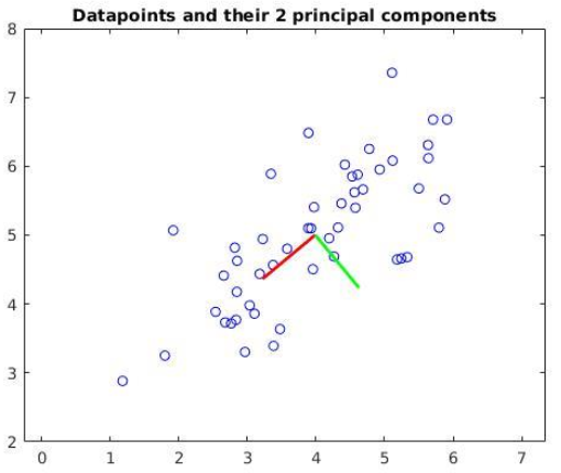
5. Add to Figure 1 the plot of the 2 principal components, in which the first component (corresponding to the largest eigenvalue) is red, and the second one is green. Your Figure 1 should look similar to Figure A below. Also print out on the command window the coordinates of the top eigenvector.

[HINT: you can use the command line to draw the eigenvector. Do not forget that the eigenvectors were calculated from data from which the mean had been subtracted. So you will need to add the mean to the eigenvectors in order to make the plot.]
6. Call a function called projectData that you will also write and include in the submission. The function receives 3 arguments: a dataset (i.e. a matrix), a set of eigenvectors and a positive integer k. It provides as the only output argument a dataset obtained by projecting the input dataset onto the first k eigenvectors. Note that the first k eigenvectors are the k eigenvectors corresponding to the k largest eigenvalues.

Your script will run this function on your dataset Xmu, using the eigenvectors in U and with k equal to 1 and obtain a matrix Z of projected data.

[HINT: here the projection of a datapoint onto an eigenvector can be obtained by calculating the dot product between the point and the vector, since the eigenvectors you obtain from Matlab have unit norm].

7. Print in the command window the projection of the first 3 points in your dataset, i.e. Z(1:3, :).

8. Call a function recoverData provided on the Moodle page. The function receives 4 arguments: a dataset (i.e. a matrix), a set of eigenvectors, a positive integer k and a vector mu. It provides as the only output argument a dataset obtained by projecting back your points onto the original space. Using the variable names described above the call in your script call would be:

Note that this function will work correctly only if the eigenvectors in U are ordered according to the size of their corresponding eigenvalues, in decreasing order, as explained in point 4.

Your script will run the above line obtaining in Xrec the recovered datapoints.

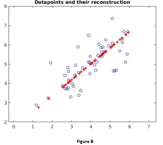
9. Create Figure 2. In this figure, plot the points as blue circles in 2D, in a figure whose axis are set in the range xmin = 0, xmax=7, ymin=2, ymax=8. Then add the recovered points as red stars. (Using the variable names described above your recovered points will be contained in the variable Xrec). Your Figure 2 should look similar to the Figure B below.

Part 2 (7 points)
In this part of the exercise you will repeat on a larger real world dataset exactly the same analysis that you have already performed on the small toy dataset. Your script will use the functions you have written for the small toy dataset. Your script will work on a dataset of 5000 images of faces of famous people, taken from a public repository. Each image is a 32x32 matrix of pixel which has been linearized into a vector of size 1024. These images are contained in the file pcafaces.mat, available on the Moodle page.
1. Load the datapoints contained in the file pcafaces.mat. Let us call X this initial set of datapoints. X has size 5000x1024, as there are 5000 faces, each represented by a vector of pixels of size 1024. (This is a large dataset so it might take a few seconds, depending on your machine).
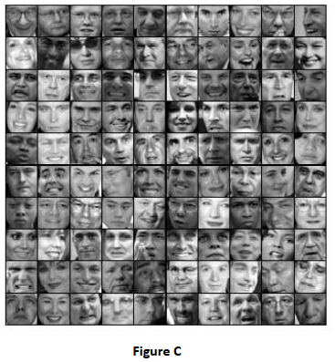
2. Create Figure 3. Use the function displayData provided on the Moodle page to display the first 100 images in the datasets. Using the variable names described above the call in your script call would
be:

displayData(X(1:100, :))

Your Figure 3 should look similar to the Figure C below.
3. Subtract the mean from X using your function subtractMean

4. Project the data onto the first 200 principal components using your function projectData

5. Recover your images back onto the original space using the function recoverData (which is provided on the Moodle page).

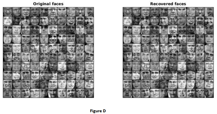
6. Create Figure 4. This figure will contain 2 subplots. The first subplot will display the first 100 images of the original data (that is, it will be the same as Figure 3). The second subplot will display the first 100 images of the reconstructed data – in this way you will be able to compare how good your reconstruction is! Your Figure 4 should look similar to the Figure D below. 

For fun, you can experiment and check the quality of the reconstructed faces for different number of principal components…

Marking Criteria

This coursework is assessed and mandatory and is worth 40% of your total final grade for this course. 

In order to obtain full marks for each question, you must answer it correctly but also completely, based on the contents taught in this course.

It will be important to provide input and output parameters to the functions as requested in the exercises. Unless explicitly specified in the exercise, avoid using the “input” function or printing outputs on the command window.

Marks will be given for writing elegant, compact, vectorised code, avoiding the use of “loops” (for or while loops) where possible, and including comments.