ECON 211 SPRING 2023 ASSIGNMENT #4 PRODUCTION AND COSTS
Hello, dear friend, you can consult us at any time if you have any questions, add WeChat: daixieit
ECON 211 SPRING 2023 ASSIGNMENT #4 PRODUCTION AND COSTS
Q1: (10 points) Let Q(L) = 12L2 – (L3)/4 with costs = 1000 + 50L.
a) (5 points) Complete the table on the next page. You can do this in excel or by hand.
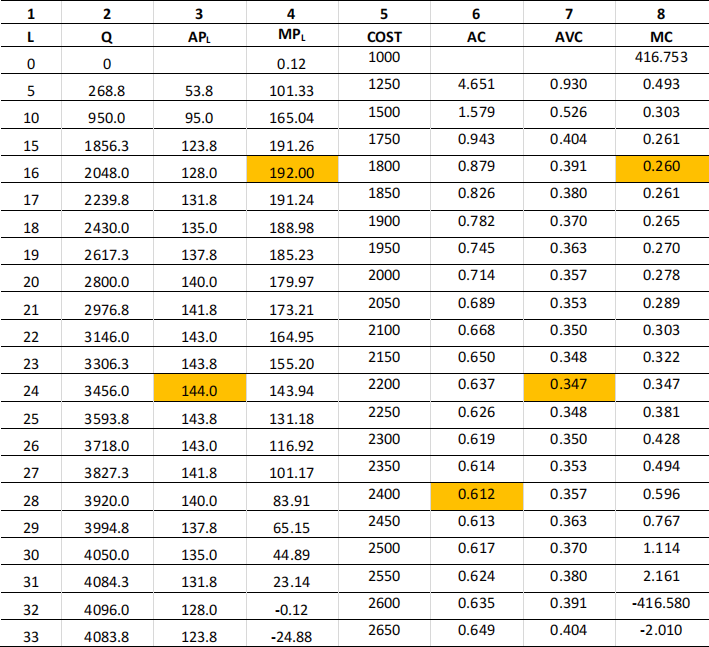
TABLE: Column 1: Labour input from 1-24
Column 2: Output resulting from L: Q(L) = 12L2 – (L3 )/4
Column 3: Average Product of Labour APL = Q/L
Column 4: Marginal Product of Labour: MP = ∆Q/∆L
Column 5: Cost: COST = 1000 + 50L
Column 6: Average Cost: AC = COST/Q
Column 7: Average Cost: AVC = (COST- 1000)/Q
Column 8: Marginal Cost: MC = ∆C/∆Q
b) (1 point) At what value of L is output maximized? (eg, the firm will never hire more than this L.)
For L=32, output is 4096. If we raise labour, say to 33, then Q=4083. Hence max output is
4096. This means the firm will never produce past L=32 since it costs more but will reduce output. It cannot be profit maximizing.
c) (1 point) Confirm that APL is maximized where MPL = APL. (You can plot APL and MPL versus L. Or you can use the table directly. Find the maximum APL. For labour below this we should see MPL > APL. For labour above we should see MPL < APL.)
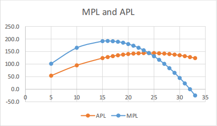
Use: scatter plot with L in first column and APL, MPL is second and third column.
Confirmed: Maximum APL is at L = 24. If L is less than this, MPL is higher than APL which raises APL . For L larger than 24, MPL is smaller and so reduces APL .
d) (1 point) d) Confirm that AC is minimized where MC = AC : if you plot this, then just show in your plot.
Minimum AC occurs at Q=3920 (L=28). If Q is less than this, MC is lower than AC which raises AC. For Q larger than 3920, MC is larger and so raises AC.
e) (1 point) Confirm that: AVC is a minimum where APL is a maximum
Minimum AVC is 0.347 and occurs at Q=3456 (L=24). APL is maximized at the same level. The idea is that AVC= wL/Q = w/(Q/L) = w/APL hence as APL rises, AVC falls (and vice versa).
f) (1 point) Confirm that: MC is a minimum where MPL is a maximum
Minimum MC is 2.60 at Q=2018 with L = 16. But this is where MPL is at a maximum of 192
Q2: (10 points) Consider a firm that employs capital and labour and uses the production technology Q = min[10K, 10L] (think of taxi cabs: you need exactly one car and one driver per taxi but each taxi can generate 10 rides per shift). Factor prices are r for capital and w for labour.
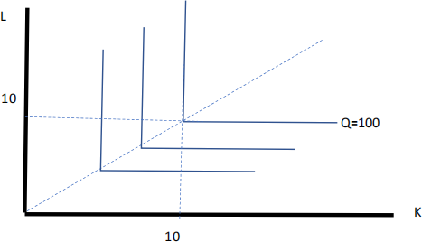
a) (3 points) Draw the isoquant for Q = 100.
Recall: an isoquant is combinations of K and L that produce Q=100.
ISSUE: inputs here are perfect complements so the Isoquant is a ‘right-angle’ . The corner is at L=10 and K=10. That is, we need to set 10K=10L or K=L. for Q=100 we have K=100/10=10
b) (1 point) Does this production function exhibit increasing, constant, or decreasing returns to scale? Show/explain.
DEFN: CRS implies a doubling of inputs will exactly double inputs.
So if we compare L=10 and K=10 with Q = 100 to L=20 and K=20 with Q=200, we see that we have CRS
c) (1 point) What is the optimal relationship between K and L? What is the input demand for Labour (L as a function of Output) and the input demand for Capital?
The optimal relationship is K = L: we use inputs one for one. Therefore input demands are K = Q/10 and L=Q/10
d) (2 point) Derive the long-run cost function: (eg C = wL + rK where L and K are optimal choices).
STEP 1: we have to find C = wL + rK for and level of output Q
STEP 2: for any Q we must have K = Q/10 and L = Q/10 C = wQ/10 + rQ/10
STEP 3: so C = Q(w+r)/10
e) (1 point) What is the long-run marginal and average cost function with r = 10 and w = 5?
MC= ∆C/∆Q = (w+r)/10 = (10+5)/10 = $1.5
AC = COST/Q = (w+r)/10 = (10+5)/10 = $1.5
Notice that since AC is constant (not rising or falling) it must be equal to MC.
f) (1 point) What is the cost of Q=100? Q= 200?
C(Q=100) = Q (15/10) = 150
Eg: to get Q=100, we need K=10 and L=10. So wL + rK = 5(10)+10(10) = 150.
Alternately C= Q * AC = 100*1.5 = 150
C(Q=200) = 300
g) (1 point) Does this cost function exhibit increasing, constant, or decreasing economies of scale?
DEFN: CES implies a doubling of output will exactly double costs.
Clearly doubling output does double costs.
Q3: (10 points) Consider the following production function: Q = K1/3 L1/3 with rental costs r and labour costs w.
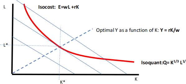
a) (1 point) Draw the isoquant for Q = 100.
Want combinations of K and L that yield Q=100. We approach this the same way that we did the Cobb- Douglas preferences.
STEP 2: isolate L1/3 : L1/3 = 100/ K1/3
STEP 3: raise both sides by power of 3 (L1/3 )3 = (100/ K1/3 )3
STEP 4: simplify: L = 1003/ K
STEP 5: create table of K and L (and check that Q = 100)

b) (1 point) Does this production function exhibit increasing, constant, or decreasing returns to scale? Show/explain.
We have Decreasing Returns to Scale:
Step 1 Set K = 100 and L = 10,000 so Q = 100 from table
Step 2 Now double K and L: Set K = 200 and L = 20,000 hence Q = 158 .
Step 3: since Q increases but by less than double, we have DRS
c) (1 point) Let K be variable. What is the optimal relationship between K and L: (hint: MRTS = L/K)
Optimality (tangency between the isoquant and the isocost line) implies Y = rK/w
STEP 1 Optimality requires MRTS = r/w where MRTS = MPK / MPL
STEP 2 MPK = ⅓ K1/3 – 1 L1/3 and MPL = ⅓ K1/3 – 1 L1/3
STEP 3 so MRTS = [⅓ K1/3 – 1 L1/3 ]/[ ⅓ K1/3 – 1 L1/3 ] = L/K
STEP 4: now set to = r/w L/K = r/w or L = rK/w
d) (2 points) What is the input demand for Labour (as a function of Output) and the input demand for Capital?
Need to substitute the optimality condition back into the production function to get K as a function of Q and L as a function of Q
STEP 1 sub Y = rK/w Q = K1/3 L1/3 = K1/3 (rK/w) 1/3
STEP 2 simplify Q = K2/3 (r/w) 1/3
STEP 3 isolate K2/3 K2/3 = Q (w/r) 1/3
STEP 4 raise both sides to power (3/2) K* = Q3/2 (w/r) 1/2
This is the input demand for K: if Q rises we need more K; if r rises we use less K; if w rises, we
use more K
STEP 5 sub into Y = rK/w L = (r/w) Q3/2 (w/r) 1/2
STEP 6 simplify L* = Q3/2 (r/w) 1/2
This is the input demand for L: if Q rises we need more L; if r rises we use more L ; if w rises, we use less L
e) (1 point) Derive the long-run cost function. (eg C = wL + rK where L and K are optimal choices).
All we do is substitute L* and K* into C= wL* + rK*
STEP 1 substitute C = w[Q3/2 (r/w) 1/2 ] + r[Q3/2 (w/r) 1/2 ]
STEP 2 simplify C = Q3/2 r ½ w ½ + Q3/2 r ½ w ½
STEP 2 simplify more C = 2 Q3/2 r ½ w ½
Notice: costs rise if Q rises, if r rises, or if w rises.
f) (1 point) Plot the cost function given w = $10 and r = $10.
From above: C= 2 Q3/2 (10) ½ (20) ½ = 93.91
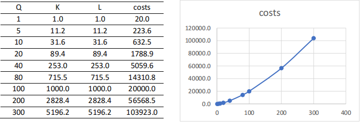
g) (1 point) Calculate the long-run costs for Q = 100. Q = 200.
See above table: C(Q=100) = 20,000 and C(Q=200) = 56,568
h) (2 points) Does this cost function exhibit increasing, constant, or decreasing economies of scale? Why does this happen?
As we can see, a doubling of output more than doubles costs. The reason is that we have DRS. To double output we need to more than double inputs. Eg to go from Q=100 to Q=200 we need to raise K from 1000 to 2828 and L from 1000 to 2828.
TOTAL: 30 points
2023-06-26