Exercise 1. Bayesian network (Homework)

Consider the Bayesian network below where all variables are binary:

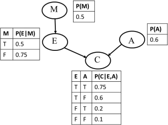
Compute the following probability and show your calculations: P(M=T, E=T, A=F, C=T).

Solution:

P(M=T, E=T, A=F, C=T) = P(m, e, ~a, c)=P(m)P(e|m)P(~a)P(c|e,~a)=0.5*0.5*(1-0.6)*0.6=0.06

Exercise 2. Probabilistic reasoning

Consider the dental example discussed at the lecture; its full joint probability distribution is shown below:

Calculate the following:

a)  P(toothache)

b)  P(Cavity)

c)   P(Toothache |cavity)

d)  P(Cavity| toothache  catch)

Solution:

a)  P(toothache)=P(Toothache=true)=0. 108+0.012+0.016+0.064=0.2

Note that:

toothache is a shorthand for Toothache=true and

~toothcahe is a shorthand for Toothache=false

b)  P(Cavity) is the probability distribution of the variable Cavity – i.e. a data structure, containing the probability for each value of Cavity. As Cavity has 2 values (true and false), P(Cavity) will have 2 elements – 1 for Cavity=true and 1 for Cavity=false. For binary variables, by convention, the first element is for true.

P(Cavity) = < P(Cavity=true), P(Cavity=false) >=

=< (0. 108+0.012+0.072+0.008), (0.016+0.064+0. 144+0.576) >=<0.2, 0.8>

c)   P(Toothache |cavity) =

=< P(Toothache=true | Cavity=true), P(Toothache=false | Cavity=true) > =

=< P(toothache | cavity), P(~toothache | cavity) >

Method 1: Without  (i.e. by calculating the denominator)

Let’s compute the first term:

P(toothache | cavity)=

= P(toothache, cavity)/P(cavity)= (from the def. of conditional probability: P(A|B)=P(A,B)/P(B) ) =(0. 108+0.012)/(0. 108+0.012+0.072+0.008)=0. 12/0.2=0.6

Now the second term:

P(~toothache | cavity)=

=P(~toothache, cavity)/P(cavity)=(0.072+0.008)/0.2=0.08/0.2=0.4

=> P(Toothache |cavity) =<0.6, 0.4>

Method 2: With  (i.e. without calculating the denominator)

Let’s compute the two terms in another way, using the normalization term :

P(toothache | cavity)=  P(toothache, cavity)=

= (0. 108+0.012) = *0. 12

P(~toothache | cavity)=  P(~toothache, cavity)=

= (0.072+0.008) = *0.08

=> P(Toothache |cavity) =<0. 12, 0.08>

Computing the normalization term: 0. 12+0.08=0.2

=> P(Toothache |cavity) =<0. 12/0.2, 0.08/0.2> =<0.6, 0.4>

d)  P(Cavity| toothache 八 catch) = < P(cavity| toothache 八 catch), P(~cavity| toothache 八 catch) >

Here we will do it without ; you can do this with  as an exercise at your own time.

Let’s compute the first term:

P(cavity| toothache 八 catch) = P(cavity, (toothache 八 catch))/P(toothache 八 catch)

Computing the denominator: P(toothache 八 catch)=0. 108+0.012+0.016+0.064+0.072+0. 144=0.416 => P(cavity| toothache 八 catch)=(0. 108+0.012+0.072)/0.416=0.4615

Now the second term:

P(~cavity| toothache 八 catch) = P(~cavity, (toothache 八 catch))/P(toothache 八 catch)= 

b)  The CPTs are:

For node Storm (S):

For node Burglar (B):

For node Cat (C):

For node Alarm (A):

c)  We need to compute P(A=true| S=true).

 P(a, s, Bb , Cc)

P(a, s)      b,c                         

P(s)                  P(s)

B and C are the hidden variables;  Bb means summation over the different values B can take.

b

Computing the numerator:

P(a | s) =  P(a, s, Bb , Cc) =

b,c

=  P(a | Bb , Cc)P(s)P(Bb | s)P(Cc | s) = b,c

= P(s) P(a | Bb , Cc)P(Bb | s)P(Cc | s) = b,c

= P(s)[P(a | b, c)P(b | s)P(c | s) +

P(a | b,」c)P(b | s)P(」c | s) +

P(a | 」b, c)P(」b | s)P(c | s) +

P(a | 」b,」c)P(」b | s)P(」c | s)] =

= 0.31*[1* 0.25 * 0.75 +   0.67 * 0.25 * 0.25 + 0.25 * 0.75 * 0.75 + 0.2 * 0.75 * 0.25] =

Using the Bayesian network assumption

Moving P(s) out of the summations

We have 4 sums, for:

b,c

b,~c

~b,c

~b,~c

= 0.31*(0. 1875 + 0.0418 + 0.1406 + 0.0375) =

= 0.1263

The denominator: P(s)=0.31 (directly from CPT)

=> P(a | s) =  =  = 0.4035

Task: As an exercise at home, compute the same probability using  .

Note: We can slightly reduce the calculations by separating the two summations and pushing the summation over c in, like this:

P(a | s) =  P(a, s, Bb , Cc) =

b,c

=  P(a | Bb , Cc)P(s)P(Bb | s)P(Cc | s) = b,c

= P(s) P(Bb| s) P(Cc | s)P(a | Bb , Cc) =       <- Pushing the summation over c in: b                   c

= 0.31* P(Bb | s)[0.75* P(a | Bb , c) + 0.25 * 0.25* P(a | Bb ,  c)] =   <- Summation for c and ~c b

= 0.31*[0.25* (0.75*1+ 0.25* 0.67) + 0.75* (0.75* 0.25 + 0.25*0.2)] =  <-Summation for b and ~b

= 0.31* (0.25* 0.9175 + 0.75* 0.2375) =

= 0.31* 0.4075 =

= 0. 1263

p(a, s)       0. 1263

P(a | s) =                  =                  = 0.4074

P(s)         0.31

Exercise 4. Using Bayesian networksfor classification

The figure below shows the structure and probability tables of a Bayesian network. Battery (B), Gauge (G) and Fuel (F) are attributes, and Start (S) is the class. If the evidence E is B=good, F=empty, G=empty, which class will the Bayesian network predict: S=yes or S=no?

Hint: Compute the joint probabilities P(E, S=yes) and P(E, S=no), normalize them to obtain the conditional probabilities P(S=yes|E) and P(S=no|E), compare them and take the class with the higher probability as the class for the new example.

Solution:

1) Computing P(E, S=yes) and P(E, S=no):

P(E, S=yes)=P(B=good, F=empty, G=empty, S=yes)=

=P(B=good)P(F=empty)P(G=empty|B=good,F=empty)P(S=yes|B=good,F=empty)

As P(B=bad)=0. 1 => P(B=good)=1-0. 1=0.9

P(S=yes|B=good,F=empty)=1-0.8=0.2

=>P(E,S=yes)=0.9*0.2*0.8*0.2=0.0288

Similarly:

P(E, S=no)=P(B=good, F=empty, G=empty, S=no)=

=P(B=good)P(F=empty)P(G=empty|B=good,F=empty)P(S=no|B=good,F=empty)=

=0.9*0.2*0.8*0.8=0. 1152

2) Normalisation:

P(S=yes|E)=0.0288/(0.0288+0. 1152)=0.0288/0. 144=0.2

P(S=no|E)=0. 1152/(0.0288+0. 1152)=0.8

3) Decision:

As 0.8>0.2, the Bayesian network predicts class no for the new example.

Another way to solve this – a smarter way for our example:

We need to compute these 2 conditional probabilities and compare them:

P(S=yes| B=good, F=empty, G=empty)

P(S=no| B=good, F=empty, G=empty)

We know the values of the parents B and F (B=good, F=empty). The Bayesian network assumption says that “A node is conditionally independent of its non-descendants, given its parents” . So if we know the values of the parents, the value of G is irrelevant (S is conditionally independent of G), i.e.:

P(S=yes| B=good, F=empty, G=empty) = P(S=yes| B=good, F=empty)

P(S=no| B=good, F=empty, G=empty) = P(S=no| B=good, F=empty)

And we already have the values of these 2 probabilities from the CPT:

P(S=yes| B=good, F=empty)=1-0.8=0.2

P(S=no| B=good, F=empty)=0.8

Hence: P(S=yes| B=good, F=empty, G=empty)=0.2 and P(S=no| B=good, F=empty, G=empty)=0.8. All done – no calculations at all in this case!

Exercise 5. Using Weka – Naïve Bayes and Bayesian networks

Load the weather nominal data. Choose 10-fold cross validation. Run the Naïve Bayes classifier and note the accuracy. Run Bayesian net with the default parameters. Right-click on the history item and select Visualize graph. This graph corresponds to Naïve Bayes classifier, that’s why the accuracy results are the same. This is because the parameter maximum_number_of_parents_of_a node is set to  1 in the K2 algorithm used to automatically learn the Bayesian network. Change it to 2 (for example) and a more complex Bayesian net will be generated and the accuracy will change (improves in this case).