Hello, dear friend, you can consult us at any time if you have any questions, add WeChat: daixieit

EENG30010 - Mobile Communication Systems

Mobile Communications Systems – Part 1

2020-21

Coursework 1 Instructions

For this coursework you need to write a technical note with detailed answers to the three questions. Additionally, for the question Q1.3 you need to submit a MATLAB script that was used to plot your results. The marking schemes and the deadlines are at the end of this instruction sheet.

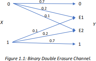
Q1.1: Compute the capacity for the Binary Double Erasure Channel given in Figure 1.1. Provide all main steps in the answer.

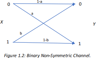
Q1.2: A binary non-symmetric channel is shown in Figure 1.2. Compute the capacity for this channel as a function of the error probabilities P(Y = 1|X = 0) = a, P(Y = 0|X = 1) = b . Provide all main derivation steps in the answer.

Q1.3: Compute the capacity of the MIMO wireless channel for the case where the channel is assumed to be an identity matrix I. Assume Gaussian signalling input X, and Addictive White Gaussian Noise

Write in MATLAB a code that plots the capacity curves vs SNR for the cases when nT = nR = 6, 12, 24. Compare the results with the case where the individual channels in the wireless MIMO system are all independent and iid complex circular symmetric Gaussian  When comparing the results scale the channels in the unitary case, so that the average energy in the channels is the same for both cases. Discuss your results.

Marking scheme

The total for the Coursework 1 is 50 marks, which is split as follows:

Q1.1: 10 Marks

Q1.2: 20 Marks

Q1.3: 20 Marks

Mobile Communications Systems – Part 2

Introduction and getting started

1 Introduction

Part of this coursework will be performed using MATLAB software on a PC/laptop and part will consider the design of mobile communication systems.

2 Getting Started

Before you can start MATLAB for windows, you must ensure that you are in the windows environment. Now double clicking on the MATLAB icon will launch MATLAB and cause a Command window to be opened with a >> prompt. The >> prompt sign means MATLAB is waiting for your input and you can type the required commands for execution.

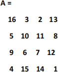
For example to enter a matrix A, simply type in the Command Window

MATLAB displays the matrix you just entered:

When you want to leave MATLAB, type exit. However if you want to stop but would like your results to be saved for the next session you need to use save to store all your variables. See Matlab help for further details on save and load.

save FILENAME saves all workspace variables to the binary "MAT-file" named FILENAME.mat.

3 Demo

An interesting way to learn the features of MATLAB is through the MATLAB demonstration. Type demo and the demo menu will be displayed. You can select the demos of interest and follow the instructions.

4 Graphical Output

MATLAB graphics system provides a variety of sophisticated techniques for visualising data. The basic syntax is plot(x,y,'linetype') which plots vector y against vector x with the specified linetype (colour and marker).

For example to plot the first 100 elements of s type

s=randn(100,1);

plot(s(1:100))

The plot appears in a separate graphics window. We can add labels and title to this plot by typing

xlabel('Sample #'), ylabel('Amplitude '), title('A random signal ')

semilogy is a Semi-log scale plot. For example you can use it later on to plot BER curves:

semilogy(EbNo,ber,'*'); Type help semilogy for more information

5 AWGN

There are a number of ways to add awgn to your simulation. Below are some useful functions:

randn creates normally distributed random numbers.

Example n=sigma* (randn(50000,1)+j*randn(50000,1)); where sigma is the standard deviation of the noise

Example: sigma=sqrt(1/(2*SNR)); %standard deviation of AWGN

awgn adds white Gaussian noise to a signal. Type help awgn

berawgn gives the Bit error rate (BER) for uncoded AWGN channels (theoretical curve). The berawgn function returns the BER of various modulation schemes over an additive white Gaussian noise (AWGN) channel. The first input argument, EbNo, is the ratio of bit energy to noise power spectral density, in dB. If EbNo is a vector, the output ber is a vector of the same size, whose elements correspond to the different Eb/No levels.

Syntax

ber = berawgn(EbNo,'qam',M). Type help berawgn

6 Random Data

randint generates a matrix of uniformly distributed random integers. This will be useful to create your random data (example 10000 data bits). You can then modulate the data (BPSK or QPSK). For example a QPSK symbol might be 1+j*1.

Syntax

out = randint(1,m) where m is the number of random integeres

7 Rayleigh fading

berfading gives the theoretical Bit error rate (BER) for Rayleigh and Rician fading channels. See Matlab help for further details.

Coursework Part 2

The total for the Coursework 2 is 50 marks.

Q2.1 Coursework assignment using Matlab (30 marks)

a) Plot the theoretical error probability for BPSK, QPSK and 16QAM in AWGN for different Eb/No values. Explain why the performance of 16QAM is worse than QPSK. Comment on the data rates/spectral efficiency they can provide

Note: For this part, you can use the functions provided by Matlab (see above) or write your own code based on the equations for the theoretical error probability that can be found in your notes and a number of books.

b) Write a program in Matlab to perform a baseband simulation of a QPSK communication system in AWGN and compare the performance with the theoretical curves above (create some random data to be transmitted). Explain the structure of the code and justify the matlab functions and parameters used.

c) Plot the theoretical error probability for QPSK and 16QAM in Rayleigh fading. Discuss Rayleigh fading and the key concepts of fast fading. Describe what is the difference between Rayleigh and Ricial fading.

d) Use diversity to improve performance in Rayleigh fading. Plot the error probability for QPSK and 16QAM in Rayleigh fading with diversity orders of 2 and 4 using ber = berfading(EbNo,'pam',M,divorder)

Discuss and compare different types of diversity and how they can improve performance of communication systems in fading channels.

e) Discuss your results and suggest other methods to improve the performance in AWGN or Rayleigh fading environments.

Q2.2 Cellular planning (10 marks)

A digital microcellular system has 30MHz of available spectrum and operates with a cluster size of 7. Each channel requires 200 kHz of spectrum. The radio system uses TDMA with 8 calls per channel. Assume that each user represents a traffic load of 0.02 Erlangs. The cell radius is 160m, and the network comprises 40 basestations.

a) What is the channel bandwidth?

b) What is the maximum number of calls that can be supported in a cell?

c) How many subscribers can we have per cell?

d) What is the maximum number of calls that can be supported in a cluster group?

e) What is the cluster area?

f) Determine the total capacity in terms of calls per MHz per kilometre square.

g) Determine the subscriber capacity in terms of subscribers per MHz per kilometre square.

h) What is the total subscriber capacity of the network? 6

i) What is the total coverage area?

j) Why microcellular systems offer higher capacity?

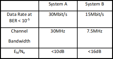
Q2.3 System design (10 marks)

a) With the aid of the graph given in the figure below, indicating the performance of various digital modulation schemes operating in an (AWGN) channel with an error rate of 10-5 , select suitable modulation schemes in order to meet the following criteria.

b) With the aid of the same graph explain why QPSK can offer a throughput enhancement compared to BPSK without either a bandwidth expansion or an increase in transmission power? In addition discuss why the noise performance of QPSK is superior to 8PSK and 16QAM is superior to 16PSK.