Hello, dear friend, you can consult us at any time if you have any questions, add WeChat: daixieit

Examination Paper For STAT0015

STAT0015: Medical Statistics 2

2020 Solutions

Q1

a) The condition of the patient needs to be similar at the start of both cross-over periods, i.e. the treatment should not cure the patient.

b) The ratio (parallel/cross-over) of sample size is

Therefore, the required sample size is

c) The most appropriate method is block randomisation with random block sizes. First randomly choose the block size, then randomly choose a pattern corresponding to that block size. Patients should be randomised to either A-B or B-A (where one group is pioglitazone hydrochloride and the other is control).

The list should show patients randomised to either A-B or B-A and should be consistent with the specification.

Q2

a) An imputation model is specified that relates blood pressure at 6 months to other variables including blood pressure at 3 months.

This model is used to generate several possible ‘imputed’ datasets where blood pressure at 6 months has been imputed.

Each dataset is analysed separately, producing an estimated treatment effect which are then combined using Rubin’s rules.

b) The baseline characteristics of patients with and without 6-month outcome data in each trial group could be summarised to investigate whether the balance of trial has been affected by the missing data.

In addition, it would informative to summarise the 3 month outcome data in these patients to investigate whether patients who are not responding to treatment are more likely to drop-out.

Q3

a) The stopping rule for efficacy should be based on O’Brien-Fleming,. e.g. “The study should stop for efficacy if the trial is statistically significant at the 0.5% level in favour of dutasteride”.

This choice preserves both the type 1 error and the power.

b) The recommendation would be to continue the trial since there is not quite enough evidence to stop the study for efficacy.

Q4

a) Use the formula where

This gives n=14 (rounded up from 13.98)

b) To obtain a trial success you need 4 improvements in the first stage and more than 13 in the second.

Under the null

Under the alternative

c) The probability of continuing at stage 1 under the null hypothesis is

Therefore the expected number is

Q5

a) First calculate the SEs of each estimate (by dividing the range of the confidence intervals by 2x1.96=3.92) then calculate the weights as the inverse of the square of these SEs.

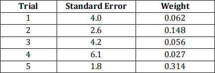
The estimate is the weighted sum of the mean differences: -4.49

The SE is sqrt(1/sum(weights)) = 1.29

This can be used to construct the interval -7.0 to -2.0

Therefore, exposure to -blockers reduces respiratory function by -4.5 units on average.

There is strong evidence that this is a real effect (CI excludes 0).

Q6

a)

Therefore:

b) The baseline survivor function at five years (60 months) is:

Therefore the survivor function for this patient is:

So the risk of ICH within 5 years is 0.317.

c) The PH assumption could be investigated using a log-log plot which plots the log cumulative hazard against time for groups of patients.

Age would need to be categorised for this plot. One possibility is to split age in three groups (e.g. based on tertiles) and produce separate plots for age (group) and microbleeds (absent/present).

If the PH assumption holds for this model we would expect to see parallel, straight lines.

d) There are seven comparable pairs: 1 vs all, 3 vs 4 & 5, 4 vs 5

Six of these are concordant (3 vs 4 isn’t) so the c-index is 6/7 = 0.857

Q7

a) Two from:

(Potentially) increased power / decreased sample size;

Allows investigation of trends over time;

Can help alleviate problems due to missing outcome data.

b) The mean response (over the 28 time-points) may be calculated for each patient. A two-sample t-test may then be performed to compare the average of these means in each trial group.

A weighted test will be required as patients supply different amounts of outcome data.

c) Suitable correlation structures include exchangeable and auto-regressive. Description of exchangeable/auto-regressive correlation with notation. exchangeable: (within-patients) 28×28 matrix with off-diagonal terms auto-regressive: (within-patients) 28×28 matrix with off-diagonal terms , , , etc.

Justification of choice:

exchangeable: all measurements within a patient assumed to be equally correlated.

auto-regressive: measurements closer in time assumed to be more correlated.

Q8

a) Plug in the numbers to get the predicted log-odds = -1.707

Convert to risk = 0.154

b) The calibration slope is a fair bit less than the one which suggests that the original model was overfitted.

The calibration in the large is greater than 0 suggesting that the predictions are, on average, slightly too low.

c) The ROC curve should show sensitivity (Y) versus 1-specificity (X) and should go through the points: (0,0), (0.474, 0.679), (1,1)

The c-statistic is the area under the ROC curve and is given by:

c = 0.5 × (1 − 0.526) × 0.679 + 0.526 × 0.679 + 0.5 × 0.526 × (1 − 0.679) = 0.5 × (0.526 × 0.679) = 0.6025

d) The PPV values are relatively low because the outcome prevalence is low. That is, most patients survive to 30 days.

Q9

a) Observations on patients within a hospital might not be independent.

If we ignore this clustering in analysis, the inference (e.g. SEs / CIs / P-values) will be incorrect. (Estimates may also be affected.)

b) One possibility is (i = hospital, j = patient):

where

c) Patients within a hospital have a 23% reduction (exp(−0.261) = 0.77) in the risk of a coronary event if they’re on treatment compared to placebo (i.e. cluster-specific interpretation).

There is evidence for an effect of treatment (95% CI does not include 0) and we’re 95% confident that the reduction is between 4% (exp(−0.041) = 0.96) and 39% (exp(−0.494) = 0.61).