(1)  If outputs are strongly disposable, then:

(a) they are also weakly disposable.

(b) there is ’no free lunch’ .

(c) output sets are bounded.

(d) All of the above.

(e)  None of the above.

(2) Suppose the output distance function takes the form DO(t)(x,q, z)  =  Q(q)/[A(t, z)F (x)]

where t is a time index, x is a vector of inputs, q is a vector of outputs, and z is a vector of environmental variables. The associated shadow revenue shares:

(a) do not depend on inputs.

(b) do not depend on environmental variables.

(c) do not change over time.

(d) All of the above.

(e)  None of the above.

(3)  If firms are price takers in input markets, then cost functions are linearly homogeneous in:

(a) output quantities.

(b) output prices.

(c) environmental variables.

(d) All of the above.

(e)  None of the above.

(4) Computing measures of output quantity change involves assigning numbers to baskets of outputs.  Measurement theory says that so-called output index numbers must be

(a) computed using output prices as measures of relative value.

(b) assigned in such away that the relationships between the numbers mirror the relationships between the baskets.

(c) superlative.

(d) All of the above.

(e)  None of the above.

(5) An analyst has obtained data on the quantities of two outputs for five firms over five time periods.  She has then used R to obtain the results presented in Figure 1.  The geometric Young index number that compares the outputs of firm 5 in period 5 with the outputs of firm 1 in period 1 is:

(a) 24.751.

(b) 27.304.

(c) 28.285.

(d) 28.979.

(e)  None of the above.

(6) An analyst has used five indices to measure changes in the input quantities reported in the first two columns of Table 1. The only proper index numbers are those reported in:

(a) columns A and B.

(b) column C.

(c) column D.

(d) column E.

(e)  None of the above.

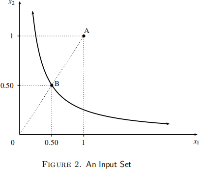
(7) Consider an industry in which firms use two inputs to produce three outputs.  The set of inputs that can  produce  a given output vector  is  depicted  in  Figure  2.   The  Lowe  index number that compares TFP at point A with TFP at point B using point B as the reference point is:

(a) 0.5.

(b) 1.

(c) 2.

(d) something that cannot be determined using the information given.

(e)  None of the above.

(8)  If a firm maximises profit, then:

(a) it must also maximise return to the dollar.

(b) it must be operating on the boundary of the production possibilities set. (c) the manager must value outputs and inputs at market prices.

(d) All of the above.

(e)  None of the above.

(9) Consider the output set depicted in Figure 3.  If (a) firms are price takers in output markets, (b) output prices are strictly positive, and (c) the price of output 1 is greater than the price of output 2, then the revenue maximising point:

(a) is point A.

(b) is point B.

(c) is point C.

(d) cannot be determined from the information given.

(e)  None of the above.

(10)  If firms are price setters in input markets and inverse demand functions are nondecreasing in inputs, then cost-minimising input combinations:

(a)  may lie above the boundary of the input set.

(b) always lie on the boundary of the input set.

(c)  may lie below the boundary of the input set.

(d) are also productivity-maximising input combinations.

(e)  None of the above.

(11) The input-oriented technical efficiency of a manager can be viewed as:

(a) a proper input index.

(b) a proper TFP index.

(c) the costefficiency of the manager divided by his/her input-oriented allocative inefficiency. (d) All of the above.

(e)  None of the above.

(12) The output-oriented mix efficiency of a manager can be viewed as:

(a) an output-oriented measure of how well he/she has captured economies of input substitution.

(b) the component of revenue efficiency that remains after accounting for output-oriented allocative efficiency.

(c) the component output-oriented technical and mixefficiency that remains after accounting for output-oriented technical efficiency.

(d) All of the above.

(e)  None of the above.

(13)  Measures of technical, scale and mixefficiency (TSME) and output-oriented technical efficiency (OTE) for six firms are reported in Table 2. The output-oriented mix efficiency of firm E is:

(a) 0.078.

(b) 0.512

(c) 1.000.

(d) something that cannot be determined from the information given.

(e)  None of the above.

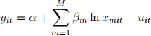
(14) Consider the following linear program:

where qit  is a vector of outputs, xit  is a vector of inputs, and zit  is a vector of environmental variables. The value of µ at the optimum is an estimate of input-oriented:

(a) allocative efficiency.

(b) mix efficiency.

(c) technical efficiency.

(d) scale efficiency

(e)  None of the above.

(15) Which of the following statements is true?

(a)  Estimates of scale efficiency can be obtained by dividing estimates of technical efficiency obtained under a VRS assumption  by corresponding estimates of technical efficiency obtained under a CRS assumption.

(b)  If  inputs  are  not  strongly  disposable,  then  the  coefficients  of the  input  variables  in locally-linear output and input distance functions are nonnegative.

(c)  If  production  possibilities  sets  are  not  convex,  then  there  is  no  linear  programming duality theory to link the primal and dual forms of piecewise frontier models.

(d) All of the above.

(e)  None of the above.

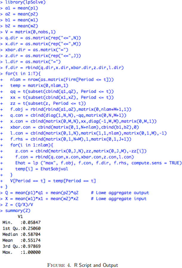
(16) An analyst  has  used data on two outputs, two  inputs and one environmental variable to analyse the performance of a group of firms.  Relevant R script and output is presented in Figure 4. The variable Z is a measure of:

(a) technical efficiency.

(b)  revenue efficiency.

(c) technical, scale and mix efficiency.

(d) environmental change.

(e)  None of the above.

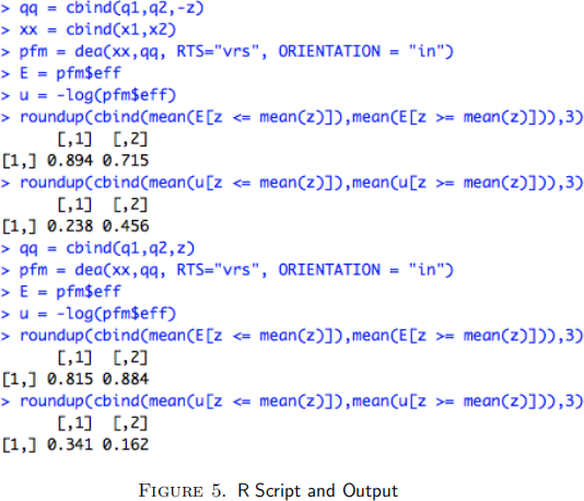
(17) An analyst has used data on two-input-two-output firms to test the null hypothesis that the average efficiency of firms operating in a relatively poor production environment (defined as an environment where the value of an environmental variable, z, is less than the mean) is no greater than the average efficiency of firms operating in a relatively favourable environment. Relevant R script and output is presented in Figure 5.  Assume the  inefficiency  effects are independent exponential random variables. The value of the test statistic is:

(a) 0.522.

(b) 1.250.

(c) 1.916.

(d) 2.105.

(e)  None of the above.

(18) Growth accountants typically assume that:

(a) input sets are homothetic.

(b) inputs are strongly disposable.

(c) technical change is implicit Hicks input neutral.

(d) All of the above.

(e)  None of the above.

(19) Consider the deterministic frontier model yit  = βo  + β1 xit  - uit   where xit   is  not random and uit  is an independent G(P, σu ) random variable with P > 2.  Which of the following statements is true?

(a) The ordinary least squares estimator for βo  is unbiased.

(b) The corrected ordinary least squares estimator for β1  is asymptotically efficient. (c) The maximum likelihood estimator for β1  is asymptotically normal.

(d) All of the above.

(e)  None of the above.

(20) Consider the following regression relationship:

yi  = 5 + 0.6 ln x1i + 0.3 ln x2i - ui

where yi  denotes the logarithm of the output of firm i, x1i  and x2i  denote inputs of capital and labour, and ui  2 0 is an output oriented technical inefficiency effect.  Consider a firm that uses one unit of capital and two units of labour to produce fifty units of output.  The output-oriented technical efficiency of the manager is:

(a) 0.237.

(b) 0.274.

(c) 0.772.

(d) 1.

(e)  None of the above.

(21) Consider the following output-oriented deterministic frontier model:

where yit  is the logarithm of the aggregate output of firm i in period t, xmit  is an input, and uit  2 0 is a random variable with the following properties:

LS1 E(uit ) = µ 2 0 for all i and t.

LS2 var(uit ) X σu(2) for all i and t.

LS3 cov(uit , uks ) = 0 if i  k or t  s.

LS4 uit  is uncorrelated with the explanatory variables.

A researcher has used R to generate the results in Figure 6.  The corrected ordinary least squares (COLS) estimate of α is:

(a) -0.485.

(b) 0.372.

(c) 1.230.

(d) something that cannot be determined from the information given.

(e)  None of the above.

(22) Which of the following statements is true?

(a) Stochastic frontier models are underpinned by the assumption that the functional forms of relevant distance, revenue and cost functions are known.

(b)  Except in restrictive special cases, stochastic frontier models cannot be used to compute primal TFP index numbers.

(c) The presence of statistical noise does not affectour ability to give an economic interpretation to the parameters in stochastic frontier models.

(d) All of the above.

(e)  None of the above.

(23) The statistical noise component in a stochastic frontier model:

(a) can generally be interpreted as a productivity index.

(b) is a normally distributed random variable.

(c) is generally  included to account for functional form errors,  measurement errors,  and

omitted variable errors.

(d) All of the above.

(e)  None of the above.

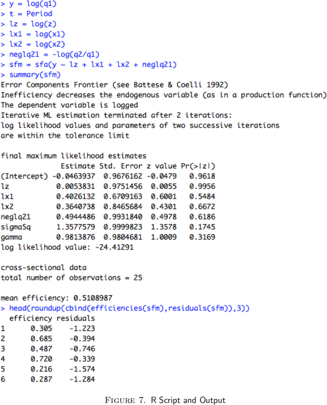
(24) Consider the following stochastic frontier model:

where qnit   is the n-th output of firm i in period t, xmit   is the m-th input, vit   represents statistical  noise,  and  uit   >  0  is  a  random  variable  representing  technical  inefficiency.   A researcher has used observations on five firms in five time periods to estimate the parameters of this model.  The results are reported in Figure 7.  She subsequently  uses these results to estimate the statistical noise component.  Her estimate of v11  is:

(a) -1.223

(b) -0.950.

(c) 0.305.

(d) 0.578.

(e)  None of the above.