J3AS 30553 Level H Applied Statistics J-BJI Semester 2 Examinations 2020-21
Hello, dear friend, you can consult us at any time if you have any questions, add WeChat: daixieit
J3AS 30553 Level H
Applied Statistics (J-BJI)
Mathematics Programmes
J-BJI Semester 2 Examinations 2020-21
1. (a) Explain two similarities and two differences between Linear Discriminant Analysis (LDA)
and Quadratic Discriminant Analysis (QDA). Use one or two sentences for each case. [4]
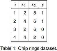
(b) Factory ”ABCD” produces very expensive and high quality chip rings. Suppose that you are a statistical consultant hired by the factory to predict whether or not a ring will pass the quality control based on its curvature and diameter. Historic data on the quality control by experts is provided in the Table 1, where x1 and x2 are the input variables, curvature and diameter respectively, y is the output (0 for failand 1 for pass) and iis the data point index.
(i) Illustrate the data points in a graph with x1 and x2 on the two axes. Represent the
points belonging to classy = 0 with a circle and those belonging to classy = 1 with
a cross. Further, annotate the data points with their data point indices. Could the
classes be well separated by a LDA classifier? Justify your answer. [4]
(ii) Suppose that the class conditional distributions f0 (x) and f1 (x) are multivariate nor- mals with means µ 0 and µ 1 respectively, where x = (x1 ,x2 )T . Assume that both classes have the same covariance matrix Σ and that the prior class probability for each class is denoted by π0for class 0 and π1for class 1. Compute the parameters of a LDA classifier using the historic data,i.e. calculate µ(ˆ)k , ![]() k and Σ(ˆ), for k = 0, 1.
k and Σ(ˆ), for k = 0, 1.
Include the calculations you have made in your answer. [5]
(iii) Derive the decision boundary for the binary classification problem stated in (b)(ii), when the decision rule is to assign an observation x to class k for which the LDA discriminant function,
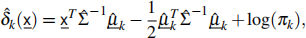
is the largest. Draw the decision boundary in the same figure as (b)(i). [4]
(iv) A new chip ring has curvature 2.95 and diameter 6.63. What is the predicted quality control outcome for a new chip ring? [1]
(c) In this problem, suppose we have a two-class setup with classes N and E , i.e. Y e {N, E}, and only one input variable X. For class N, we assume that the class conditional distribution fN (x) is Gaussian N(0, s2 ) and the prior probability is πN = Pr (Y = N) = ![]() . For the other class, the prior probability is πE = Pr (Y = E )=
. For the other class, the prior probability is πE = Pr (Y = E )= ![]() and its class conditional distribution is the exponential function given by,
and its class conditional distribution is the exponential function given by,
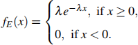
where λ > 0.
(i) Derive the decision boundary as a function of λ and s2 given that the classification rule is to classify to the class with the highest posterior probability. Show your work, starting from the posterior probabilities.
Hint: The formula for the roots of a quadratic equation in the form of ax2 +bx+c = 0, where a, b, c are constants with a ![]() 0, is given by x =
0, is given by x = ![]() . [5]
. [5]
(ii) State the assumptions of λ and s . Justify your answer. [2]
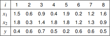
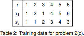
2. (a) Consider a regression problem in which there are two real-valued inputs, x1 and x2 , and a real-valued output y. The training data is given in the following table:
(i) A student constructed a regression tree displayed in Figure 1. Draw the input parti-
tioning corresponding to this tree. Make sure that you clearly mark the regions with the names of the leaf nodes R1 , R2 , R3 and R4 . [3]
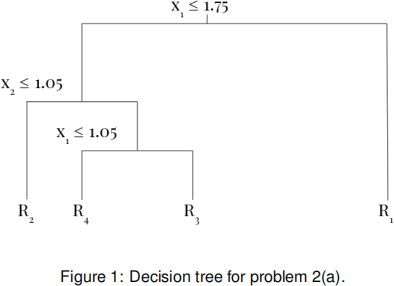
(ii) Predict the output of a new test input x* =(x1(*) ,x2(*))T =(0.8, 1.3)T . [4]
(iii) Continue to grow the tree in Figure 1 until there are at most 2 data points in each
region. Construct the additional region(s) by minimising the mean squared error. State clearly which region(s) do you split and where. [5]
(iv) Explain, using one or two sentences, the disadvantage of growing a decision tree too deep. [2]
(b) Discuss briefly two essential differences between hierarchical clustering and k-means clustering. [3]
(c) A data set with 6 observations of two variables (x1 and x2 ) is given in the Table 2. Consider the problem of clustering the data points using the k-medoids clustering algorithm. The algorithm works the same way as the k-means algorithm with the only difference being the definition of the medoid as opposed to the mean. In particular, a medoid refers to a point within the cluster for which the average Euclidean distance between it and all the other points of the cluster is minimised.
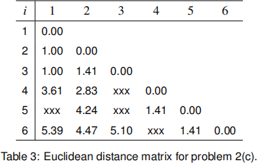
(i) The Euclidean distance matrix between the observations is given in Table 3, where
some of the values have been deleted and replaces with xxx’s. Find the missing entries. Give your answer in two decimal places. [2]
(ii) Implement the k-medoids algorithm to cluster the 6 data points into two clusters.
Use the Euclidean distance to assign each point to its nearest medoid. Show your
computations for each iteration till convergence. Suppose we initialise the k-medoids
algorithm to two initial clusters C1 = {1, 2, 3, 4} and C2 = {5, 6}, after which we run
the algorithm. In case of ties in average distance, use the data point with the smallest x1 value as themedoid. [6]
2023-06-13