Release date: Thursday, June 1st

Due date: Tuesday, June 13th, 11:59pm

Due date with your one time extension: Friday, June 16th, 11:59pm

• Questions below are either theoretical or computational. For the computational questions you may use any programming language you prefer except Maple or Mathematica. I strongly recommend using MATLAB for this assignment since otherwise you would have to reproduce the whole heat_lu_incomplete .m script.

• This assignment should be submitted to Crowdmark. Besides your written/typed solutions you  must also submit your code in either pdf or screenshot format. Please make sure your upload has the correct orientation and ordering.

• If you want to use your one time 3-day extension, please email the instructor before the original due date.

1. (0 points) Please sign the Academic Integrity Checklist (at the end of this file). If you do not sign the Academic Integrity Checklist you will receive a 0 for this assignment.

2. (theoretical, 5 points) Consider a fixed point iteration to compute the root of f (x) = 4x + cos(x) using g(x) = x − f (x) = −3x − cos(x). We want to find the only root of f (x) in [−1, 1].

(1) Compute five iterations respectively for initial guesses x0  = and x0  = − with an aid of a calculator or MATLAB and describe what you observe. Can you back up your observation with a theoretical result covered in class? You may quote the result (for example, “see [GW] theorem x.x”) without writing down the full statement but you are asked to briefly explain why the theory applies here.

(2) A more suitable g(x) is needed to remedy what occurs in (1). Consider (x) = x−H(f (x)). We claim that (x) can be used for a fixed point iteration to find roots of f (x) if H(0) = 0 and 0 is H(x)’s only root. Can you come up with an H(x) such that (x) converges? Hint: a linear H(x) = cx (c ≠ 0) would satisfy the two red conditions above immediately and you would then need to figure out a suitable c for convergence. Compute five iterations with the same initial guesses in (1) and make observations accordingly. You don’t have to theoretically justify your choice of c and you will earnfull grades with convergent iterations (to the root of f (x) in [−1, 1]).

3. (theoretical, 5 points) The phase 1 of Gaussian elimination (Algorithm 3.3 in our lecture notes) can be found in algorithm 1.  Derive that the leading order term of floating point operation count for multiplications and divisions is n3 .

4. (computational, 5 points) The heat equation is a partial differential equation that describes the diffusion of heat in a given region over time. In mathematical terms, it is expressed as

where function u(, t) is the temperature at spatial position and time t . The Laplacian Δu determines whether and how much the surrounding is hotter or colder which affects how temperature at this spatial point changes. Many numerical algorithms are designed to solve the heat equation including but not limited to Finite Difference Method (AMATH 342) and Finite Element Method (AMATH 442). For a 2D problem discretized spatially with central difference scheme and time-wise with backward Euler scheme, we end up with the following linear system to solve for each time step:

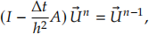(a)

where I is the identity matrix, Δt is the time step size, h is the spatial grid size and n is the

numerical solution of the temperature distribution at time t = tn . When there are 5 × 5 grid

points with Dirichlet boundary condition, the matrix A reads:

Now, you’re provided a MATLAB script heat_lu_incomplete .m1which sets up the linear system eq. (a) with Δt = h = 0.1, 19 × 19 grid points and a while loop to solve the iteration until the final time T = 1.  For every n  ≥ 1, the script solves eq. (a) with Gaussian elim- ination algorithm.  The incomplete script heat_lu_incomplete .m uses MATLAB’s built-in LU-factorization [L,U]=lu(M) and asks you to complete the phase 2 and 3 of Gaussian elim- ination (see Algorithm 3.3 from the course notes). The only lines in heat_lu_incomplete .m at which you’re asked to write codes are lines 32-33 and 39-40.

The initial temperature profile 0  (the ic vector in the script) has a hot central patch in the domain with temperature 100 degrees. When you complete the missing two chunks of code, run the script. Initial and terminal temperature profiles will be generated in subplots. Submit your code alongside with the plot.