ETF5930 Financial Econometrics
Hello, dear friend, you can consult us at any time if you have any questions, add WeChat: daixieit
Please note that the Final Exam questions are all based on (a) lecture slides and (b) tutorial questions.
Question 1
In this question we want to study whether there is a trade-off between the time spent sleeping at night and the time spent in paid work. The simple regression model can be written as
sleepi = F0 + F1 totwrki + ei
where sleep is total minutes spent sleeping at night per week and totwrk is total minutes worked during the week.
(a) If adults trade off sleep for work, what is the anticipated sign of F1 ?
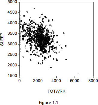
(b) Figure 1.1 gives the scatterplot of sleep against totwrk. What does this figure tell you?
(c) Figure 1.2 gives the estimation result of the regression. Write down the sample regression line. Report the results to 3 decimal points.
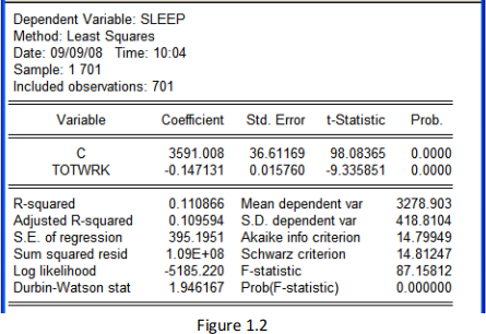
(d) Interpret the estimated intercept F0 .
(e) Interpret the estimated slope F1 .
(f) If totwrk increases by 2 hours, by how much is sleep estimated to fall?
A multiple regression model is now used to study the trade off between time spent sleeping and working and to also look at other factors affecting sleep:
sleepi = F0 + F1 totwTki + F2 educi + F3 agei + ei
where educ is years of education and age is measured in years.
(g) Do you think F2 and F3 will have obvious anticipated signs? Justify your answers.
(h) Figure 1.3 gives the estimation results. Write down the sample regression line for the multiple regression model. Report the results to 3 decimal points.
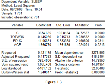
(i) Would you say totwrk, educ and age explain much of the variation in sleep?
(j) Does the estimated multiple linear regression model substantially (or greatly) improve the
goodness of fit of the model over the estimated simple linear regression model? Explain your
answer.
(k) Does including educ and age in the multiple regression model substantially (or greatly) affect the estimated trade off between sleeping and working? Explain your answer.
(l) Interpret the estimated coefficient on the educ variable.
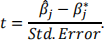
(m) Without using the p-value approach, is educ significantly related to sleep at the 5% level of significance? (Recall that z0.025 = 1.96 and z0.05 = 1.645. Also recall that
Question 2:
Figure 2.1 plots the quarterly log of U.S. real Gross Domestic Product (denoted as gdp) and log of U.S. real consumption (denoted as cons) from 1947q1 to 1980q4.

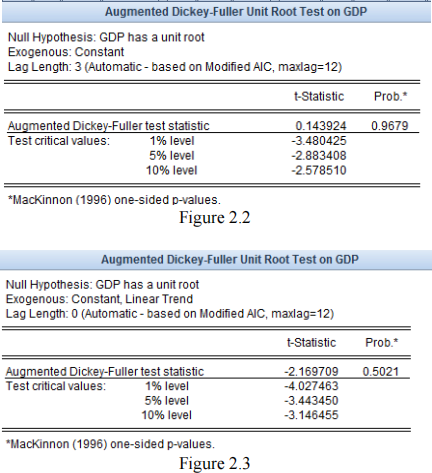
(a) EViews printouts for the Augmented Dickey-Fuller (ADF) tests for gdp are shown in Figures 2.2 and 2.3. Using only the correct EViews printout, can you conclude at the 5% level of significance that gdp has a unit root? Explain your answers by writing down the null and alternative hypotheses, the ADF regression, the test statistic, the p-value and the conclusion.
(b) Suppose that gdp and cons are both integrated of order one. A version of the permanent income theory of consumption implies the cointegrating relationship:
const = egdpt + et
where et is the cointegrating residuals. Figure 2.4 gives the Engle-Granger Augmented Dickey Fuller test for cointegration. Explain in detail, step by step, how you would investigate whether or not gdp and cons are cointegrated?

Question 3:
Suppose Yt follows the following time series model
Yt = 0.8Yt − 1 + et
where et ~i. i. d. (0,4). Let Ft = (Yt , Yt − 1, … , Y1).
(a) Compute the unconditional mean, E(Yt ).
(b) Compute the unconditional variance, var(Yt ).
(c) Compute the conditional mean, E(Yt |Ft − 1).
(d) Compute the conditional variance, var(Yt |Ft − 1).
Question 4:
A plot of quarterly Australian inflation rate (denoted as Yt ) from 1960q1 to 2006q4 is given in Figure 4.1. Let Ft = (Yt , Yt−1, Yt−2, … , Y1).

(a) The correlgoram of ∆Yt (denoted as D(Y)) is given in Figure 4.2. Explain why ∆Yt may follow an MA(1) model.

Consider an MA(1)-GARCH(1,1) model:
∆Yt = e0 + et + e e1t−1
et = at zt
at(2) = E(et(2)|Ft−1) = a0 + a1 et(2)−1 + F1 a![]() 1
1
where zt ~i. i. d. N(0, 1).
(b) The EViews printout in Figure 4.3 gives an estimated MA(1)-GARCH(1,1) model. Write down the fitted model. Express your answers in three decimal places.

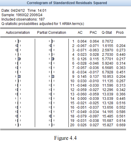
(c) Figure 4.4 is the correlogram of the squared of the standardised residuals obtained from the estimated MA(1)-GARCH(1,1) model. What does this figure tell you?
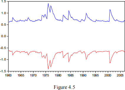
(d) Figure 4.5 plots the bands of plus and minus one conditional standard deviation based on the estimated MA(1)-GARCH(1,1) model; that is, the solid line is ![]()
![]() t and the dotted line is −
t and the dotted line is −![]()
![]() t . What does this figure tell you?
t . What does this figure tell you?
Question 5:
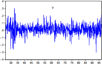
The line graph below gives the monthly log returns (denoted as yt ) from January
1926 to December 1996 for the IBM.
Part 1
The EViews printout gives the estimated AR(1)-ARCH(1) model.

(a) Write down the estimated AR(1)-ARCH(1) model.
(b) Write down the expressions for the 1-step ahead forecast, E (aT(2)+1 jFT ), and 2- step ahead forecast, E (aT(2)+2 jFT ) ; of the conditional variance for an ARCH(1) model.
(c) The within-sample-period is January 1926 to December 1996. Suppose e^T = 一0:087; where T = December 1996. Based on your answers in part (b), calculate the 1-step ahead and 2-step ahead forecast.
Part 2
The EViews printout gives the estimated AR(1)-GARCH(1) model.
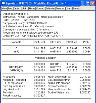
(a) Write down the estimated AR(1)-GARCH(1,1) model.
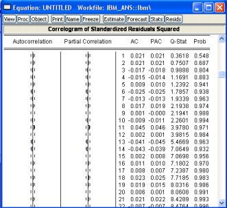
(b) The EViews printout (next page) gives the correlogram of squared residuals. Is
the estimated GARCH(1,1) model appears to be well-speciÖed? Explain.
(c) Write down the expressions for the 1-step ahead forecast, E (aT(2)+1 jFT ) ; and 2- step ahead forecast, E (aT(2)+2 jFT ) ; of the conditional variance for a GARCH(1,1) model.
(d) The within-sample-period is January 1926 to December 1996. Suppose e^T = 一0:086 and ![]() T(2) = 0:008; where T = December 1996. Based on your answers in part (c), calculate the 1-step ahead and 2-step ahead forecast.
T(2) = 0:008; where T = December 1996. Based on your answers in part (c), calculate the 1-step ahead and 2-step ahead forecast.
Question 6
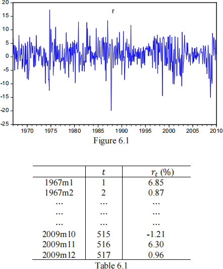
A plot of monthly log returns ( Tt ) , in percentages, of Ford stock from January 1967 to December 2009 is given in Figure 6.1. The values of Tt for the first two observations and the last three observations are given in Table 6. 1.
Suppose the log return Tt follows the AR(1) model
Tt = p0 + p1Tt − 1 + et
where et ~i. i. d. (0, G 2). Let Ft = {Tt , Tt − 1, … , T1).
(a) Derive, step-by-step, the unconditional variance vaT(Tt ).
(b) Derive, step-by-step, the conditional mean E(Tt |Ft − 1).
(c) Explain whether the following statement is true or false: “Tt is non-stationary because the conditional mean of Tt derived in part (b) is not time-invariant” .
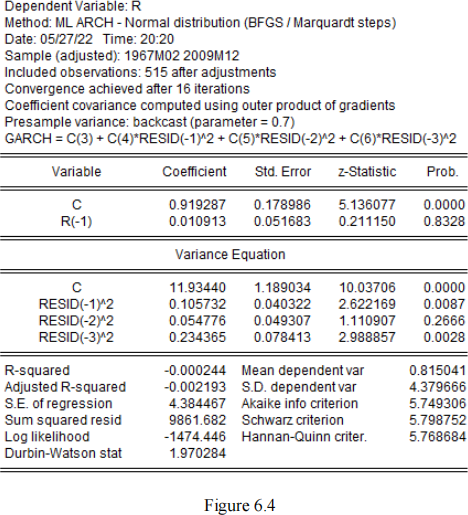
(d) Figure 6.2 gives the estimated AR(1) model. Write down the fitted model.

(e) Figure 6.3 shows the correlogram of the standardised squared residuals obtained from the estimated regression model in Figure 6.2. What does this figure tell you?

Consider the AR(1)-ARCH(3) model:
Tt = p0 + p1Tt−1 + et
et = Gt zt
Gt(2) = E(et(2)|Ft−1) = a0 + a1 et(2)−1 + a2 et(2)−2 + a3 et(2)−3
where zt ~i. i. d. N(0, 1).
(f) The estimated AR(1)-ARCH(3) model is given in Figure 6.4. Write down only the fitted conditional variance model. [1 mark]
(g) For the AR(1)-ARCH(3) model, write down the 1-step ahead forecast of the conditional mean; that is E(TT+1|FT ).
(h) Based on the within-sample period from 1967m1 to 2009m12 and the estimated AR(1)- ARCH(3) model, calculate the sample 1-step ahead forecast of the conditional mean.
(i) For the AR(1)-ARCH(3) model, derive, step by step, the 1-step ahead forecast of the conditional variance; that is E(GT(2)+1|FT ).
Question 7
Consider the monthly adjusted closing price data (denoted as Pt ) for Intel stock from January 2004 to December 2014 (obtained from the Yahoo Finance website). The values of Pt for the first two observations and the last two observations are given in Table 8.1.

(a) The simple return
2023-06-03