Instructions:

•  This test consists of 5 problem-solving questions requiring detailed solutions.

•  It is to be completed independently by each student.

•  It will count for 40% of assessment.

•  Work out the details and show the steps to solve each problem, including the right theory and methods used, appropriate formulae to calculate the answers, as well as the steps of calculations.

•  Marks for each question are shown after the question number.

•  The full marks of the assignment are 40.

•   Submit your answers in PDF file via Turnitin on iLearn by Monday 6pm, 5 June 2023.

•  The submitted answers must be typed (not handwritten).

•  Note that Turnitin requires at least 20 typed words to submit a file.

•  Resubmission is allowed before the due time.

Rules for use of R programme:

•  If a question indicates to use R, present relevant R-codes and outputs in your answers.

•  It suffices to copy-paste R-codes and outputs in your answer sheets, and not necessary to provide R-scripts.

•  Use your own words to write answers obtained from R (not just provide R-scripts).

•  For any question (or part of a question) with no mention of using R, your submitted answers should not rely on R.

Question 1   [6 marks]

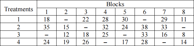
The following table presents data {Xij } in a randomized complete block design:

The null hypothesis of interest is H0 :τ1 = … = τ5 .

(a) Find the p-value of testing H0  against general alternatives H1 :τi ≠ τj  for at least one pair of (i, j) by the Friedman, Kendall-Babington Smith test and interpret the result.

(b) Calculate the approximate p-value of the Page test for H0  against ordered alternatives H2 :τ1 ≤ … ≤ τ5  with τi ≠ τj  for some i ≠ j and interpret the result.

(c) Find other ordered alternatives H3  that are supported by the data with stronger evidence than both H1 and H2  in parts (a) and (b) and explain such differences.

(d) Identify the differences between the five treatments by two-sided multiple all-treatment comparisons at an achievable level 4.5 ≤ α ≤ 5.5 . You may use R to find critical point.

Question 2   [8 marks]

Data from 4 treatments are provided below in an incomplete block design:

Consider the test of the null hypothesis H0 :τ1 = … = τ4  against general alternatives H1 by the exact rejection rule at an achievable level α ≤ 0.05 of significance.

(a) If this incomplete block design is balanced, carry out the appropriate test for DIDB. (b) Carry out the appropriate test for arbitrary incomplete block design.

(c) Compare the results in parts (a) and (b) and explain their relationship.

You may use R to find the exact critical point and calculate relevant matrices.

Question 3   [ 10 marks]

Let (X1 , Y1 ), … , (Xn , Yn ) and (X, Y) be continuous independent pairs of random variables with a common joint cumulative distribution function (cdf) F (x, y ) = Pr (X ≤ x, Y ≤ y ) .     (a) A set of data observed from (X1 , Y1), … ,(Xn , Yn ) are presented in the table below:

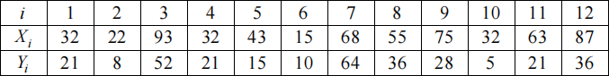
Calculate the following statistics based on the above data:

• the Kendall statistic K and

• the Spearman rank correlation coefficient r .

(b) Derive the following formula to calculate the Kendall correlation coefficient τ of the random pairs (X1 , Y1), … ,(Xn , Yn ) based on the common joint cdf F (x, y ) and the joint density f (x, y ) of (X, Y) :

τ = 4∫∫F(x, y)f (x, y)dxdy − 1 = 4E[F(X, Y)] − 1 , where f (x, y ) can be obtained from F (x, y ) via

f (x, y) =  ∂ 2F(x, y)

(c) Calculate the Kendall correlation coefficient τ by the formula derived in part (b) with the joint cdf F (x, y ) defined as follows:

(       xy                  1         

|x + y − xy = x − 1 + y − 1 − 1

|F (x,1) = x

|1          =

|

 0

if 0 < x ≤1, 0 < y ≤1;

if 0 < x ≤1, y >1;

if x >1, 0 < y ≤1;

if x >1, y >1;

otherwise (x ≤ 0 or y ≤ 0).

Question 4   [8 marks]

Use R to solve the following problems:

(a) The table below presents the data of 3 regression lines, each with 8 pairs of (x, Y) :

Let β1, β2 , β3  denote the slopes of Lines 1, 2, 3 respectively.

Find thep-value ofthe Sen-Adichie test for the null hypothesis H0 : β1 = β2 = β3  against the alternative H1  of different slopes β1, β2 , β3  and interpret the test results.

If H0  is accepted at an appropriate level of significance, use the method related to the Theil test to estimate the common slope β= β1 = β2 = β3  based on combined 24 pairs of (x, Y) ; otherwise estimate each of β1, β2 , β3  separately.

(b) The following data are drawn from a response variable Y together with four covariates

x1 , … , x4 :

Y = (36, 58, 65, 65, 70, 72, 75, 80, 82, 87, 95, 101, 102, 109, 115, 116, 118, 122, 122, 124)

x1 = (3.2, 5.3, 6.7, 6.8, 3.2, 5. 1, 3.6, 5.8, 5.7, 6.2, 5.4, 5. 1, 6.5, 5.2, 5.5, 5.0, 3.6, 4.8, 6.5, 6.6)

x2 = (51, 45, 51, 26, 64, 54, 28, 38, 46, 85, 49, 59, 73, 52, 58, 59, 74, 8, 40, 77)  x3 = (40, 23, 43, 68, 65, 56, 95, 70, 63, 28, 72, 66, 41, 73, 70, 75, 86, 79, 84, 98)

x4 = (2. 11, 2.52, 1.86, 2. 10, 0.74, 1.63, 2.33, 1.42, 1.91, 2.98, 1.84, 1.93, 2.01, 1.85, 2.64, 3.50, 3.05, 3. 15, 2.88, 1.95)

Model the data by the multiple linear regression model.

Determine which covariates have significant effects on the response at the 5% level of significance by the HM test and obtain the fitted regression model after dropping any insignificant covariate(s).

Question 5   [8 marks]

Let X1 , … , Xn  be a random sample of losses following a common continuous cumulative distribution function (cdf) F(x) , Fn (x) the empirical distribution function of X1 , … , Xn , and uα the percentile of F(x) such that F(uα ) = α .

Define the mean excess lossfunction e(u) of X ~ F(x) by

e(u) = E [X − u X > u ] = E (X − u)I{X>u } 

(a) Let X(1) ≤ … ≤ X(n)  be the order statistics of X1 , … , Xn  and k = [αn] the integer part of αn . An empirical estimate α  of uα  is given by

α =〈|X(k+1) 2

if αn is an integer

otherwise