Final Coursework

Introduction to Quantitative Research Methods (PUBL0055)

Instructions

● This is an assessed piece of coursework (worth 75% of your final module mark) for the PUBL0055 module; collaboration and/or discussion of the coursework with anyone is strictly prohibited. The rules for plagiarism apply and any cases of suspected plagiarism of published work or the work of classmates will be taken seriously.

● As this is an assessed piece of work, you may not email/ask the course tutors or teaching fellows questions about the coursework.

● Along with the coursework itself, the datasets for the coursework can be found in the PUBL0055 page on Moodle.

● Coursework should be submitted via the ‘Turnitin Submission: PUBL0055 Essay 2’ link on the course Moodle page. You will need to click the ‘Submit Paper’ link at the bottom of the page. When presented with the ‘Submit Paper’ box, the ‘Submission Title’ should be your candidate number, and you should upload your document into the box provided.

– Please remember to state ONLY your candidate number on your coursework (your candidate number is made up of four letters and one number e.g. ABCD5). Your name and/or student number MUST NOT appear on your coursework.

● The coursework consists of 8 questions. The marks allocated for each question is indicated in the text.

● Unless otherwise stated, answers should be written in complete sentences. Be sure to answer all parts of the questions posed and interpret the results.

● The word count for this assessment is 3000 words. This does not include the appendix, or any words (or numbers) contained within tables.

● Please submit your type-written (numbered) answers in a single document. Create an appendix section at the end which contains all the R code needed to reproduce your results (you do not need to include the code that failed to run, but just the cleaned-up version. Your code has to work when we run it).

● You may assume the methods you have used (e.g. difference in means, linear regression, etc) are understood by the reader and do not need definitions, but you do need to explain how they apply to answering the question.

● Round all numbers to two digits after the decimal point.

● Do not copy and paste any brute R output (e.g. lm(y ~ x)) into your answers. Create a formatted table that is easy to read.

● Assign every table and figure a title and a number and refer to the number in the text when discussing a specific figure or table.

● All variable names in the coursework are written in this_font.

The Effects of Educational Television

Is educational television an effective teaching aid? “The Electric Company” was a television programme that ran on US TV from 1971 to 1977. The programme used sketch comedy to provide an entertaining way of helping elementary school children develop their grammar and reading skills. It was widely credited by many teachers in US schools as having important effects on the literacy skills of second-, third-, and fourth-grade children. In this section, you will analyse data from an experiment that involved randomly assigning classes of children to watch “The Electric Company”. You will investigate what reading gains, if any, were made classes as part of this experiment.

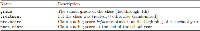
The unit of analysis in this data is a class of children, and there are 192 classes in the data. Each class was either treated (to watch the program) or control (to not watch the program). The outcome of interest is the average score on a reading test administered at the end of each year called post.score. In addition to the treatment and outcome, the data also contains information on the year grade of the class and the score on the same reading test as adminstered before the treatment took place:

The data is stored in electric-company.csv. Once you have downloaded this file and placed it in the relevant folder, it can be loaded into R as follows:

electric <- read.csv("data/electric-company.csv")

Question 1 (16 marks)

a. Calculate and interpret the average effect of the treatment on the class reading score at the end of the school year.

b. Explain whether we can interpret your answer to part a as the causal effect of television on student scores.

c. Calculate the standard error of the difference in means. Show your work.

d. Conduct a hypothesis test for the difference in means. Can we reject the null hypothesis of no effect of the treatment at the 95% and 99% confidence levels?

e. Calculate and interpret the 95% confidence intervals for the difference in means estimate.

f. Explain the concept of a “sampling distribution”. What is the shape of the sampling distribution in this example?

Question 2 (10 marks)

a. Make a scatter plot which compares student scores at the beginning of the year to student scores at the end of the year.

b. Make a box plot which depicts student scores at the end of the year as a function of the grade they are in.

c. Estimate three linear regression models. The first should predict post.score with only the treatment variable. The second regression model should be the same as the first, but should also control for student grade. The third model should be the same as the second, but should also control for pre.score.

d. Summarise these models in terms of how much of the variation in post.score they “explain”. What does this tell us about the relationships between 1) the grade a student is in and reading ability, and 2) students’ prior performance on the test and current performance on the test?

e. Are the estimates of the treatment coefficient different across the three models? Why do you think that is? You may wish to provide evidence from the data to support your argument. You may also wish to refer to your answers to parts a and b of this question.

Question 3 (6 marks)

Use the grade variable to subset the data, and then use linear regression models to evaluate the effect of treatment within each grade. How does the effect of the treatment differ as grade increases? Comment on both the substantive and statistical significance of these results.

Question 4 (6 marks)

Write a short paragraph summarising your findings from these analyses. You should write as if you are trying to communicate the results to someone who is interested in the effects of television on learning, but who has not taken a course in quantitative methods. You may wish to create a visualisation to help communicate the findings.

Political Parties and Policy Outcomes

Does which political party is in power matter for policy outcomes? This is an important question for political scientists to answer, not least because many theories of voting assume that voters hold governing parties to account on the basis of their performance in office. If such “retrospective voting” is to occur, it must be the case that different political coalitions have clear and consistent effects on policy outcomes in the time between elections.

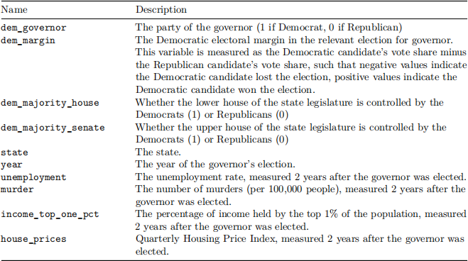
To determine whether this is the case, in this section you will use data from the US to analyse the effects of the party in power in US state governments (specifically, which party holds the governorship of the state) on a number of different policy outcomes. The data comes from 864 elections across 50 states in the US, plus the District of Columbia. The variables included in the data are:

The data is stored in governors.csv. Once you have downloaded this file and placed it in the relevant folder, it can be loaded into R as follows:

governors <- read.csv("data/governors.csv")

Question 5 (6 marks)

a. For each of the 4 outcome variables, estimate a linear regression where dem_governor is the only explanatory variable. Present the results in a table.

b. Interpret the regression coefficients in each model.

Question 6 (13 marks)

a. Adapt the regression models that you estimated above to include two additional control variables: dem_majority_house and dem_majority_senate. Estimate these regression models and present the results in a table.

b. Why might it be important to include these additional variables in your regression?

c. Interpret each of your four regressions, paying particular attention to the coefficient associated with the dem_governor variable. Can the coefficient be interpreted causally in these models? Explain why or why not.

d. Your goal is to identify the causal effect of Democratic governors on these outcome variables. Imagine that you had unlimited time and unlimited budget: describe one variable that you would ideally control for in these models. Why?

Question 7 (18 marks)

In the paper on which this example is based, the authors use a regression discontinuity (RD) design. In this design, the authors use the Democratic candidate’s electoral margin variable to make comparisons between states that narrowly elected a Democrat to states that narrowly elected a Republican for governor. In this question, you will replicate parts of the original RD analysis.

a. Write a short paragraph discussing why using a regression discontinuity design of this type might be better than simply comparing states that have Democratic governors to states that have Republican governors. Explain also one disadvantage of using a regression discontinuity design in the context of this study.

b. Use the dem_margin variable to compare policy outcomes between states that narrowly elected a Democratic governer and states that narrowly elected a Republican governor. Report and interpret the regression discontinuity treatment effect for all four outcome variables.

c. Produce four plots that depict the regression discontinuity design graphically. Each plot should depict the relationship between the Democratic electoral margin and one of the policy outcomes. Your plot should include two lines depicting the relationship on either side of the cutoff, and a vertical line to show the location of the cutoff on the x-axis.

d. Write a short paragraph which compares your findings from the regression discontinuity design analysis here to your findings from the regressions that you estimated in questions 1 and 2. What do you conclude about whether political parties have important effects on policy outcomes?

Religion and the Electoral Success of the Nazi Party in 1932

In Weimar Germany, the Catholic Church vehemently warned ordinary parishioners about the dangers of extremist parties. During this period, the church in Germany was particularly active in discouraging Catholics from supporting the Nationalsozialistische Deutsche Arbeiterpartei (NSDAP), which is commonly known in English as the Nazi party. Alerted by the Nazis’ sudden success at the polls and afraid of anticlerical movements within the party, Catholic bishops took an explicit anti-Hitler stand in the autumn of 1930. Historians have long contended that this anti-Nazi position from Catholic religious leaders had consequences for the level of support amongst Catholic citizens, particularly in the context of the Reichstag elections in 1932.

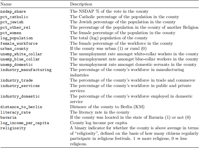
In this section, you will investigate whether Catholic areas of Germany were less likely to support the Nazi party in the elections held in November 1932. The data includes election results from 982 counties, and includes a number of variables:

The data is stored in reichstag.csv. Once you have downloaded this file and placed it in the relevant folder, it can be loaded into R as follows:

reichstag <- read.csv("data/reichstag.csv")

Question 8 (25 marks)

Your task in this section is to investigate the relationship between the share of Catholics in a district and the NSDAP vote share in that district in the election in order to answer the research question outlined above. In particular, you should implement two linear regression models with nsdap_share as the dependent variable.

In the first model, the only explanatory variable should be the pct_catholic variable. For the second model, you should build a model which – in addition to the pct_catholic variable – includes exactly three additional explanatory variables that you think might be useful to include from the supplied dataset. You should explain why you think these particular variables are important to include, given that our main interest is in the relationship between Catholicism and Nazi vote share. Please note that, for the second model, you should not estimate several different models and present the results, but rather you should argue theoretically why you chose certain variables.

You should write up the results of these models as if they were to be published in a political science journal article with a focus on communicating the substantive meaning of your results. In your discussion of these models, you should focus on communicating the substantive implications of the regression that you implement, paying particular attention to the relationship between the Catholic population of a district and Nazi vote share in the election. You may wish to focus on the following:

● Provide descriptive statistics and/or plots to provide the reader with an overview of the dependent variable and the important explanatory variable(s) that you intend to use.

● Provide a well-formatted table of regression output which includes the key information about the models you have estimated.

● Discuss both the statistical and substantive significance of the relationships that you illustrate.

● Discuss model fit, using appropriate statistics.

● Discuss whether or not we should consider the estimates you present to be causally identified.

● Discuss weaknesses of you analysis, and potential alternative analysis designs that you might use (given different data) to evaluate this research question.