Introduction

We have entered the era of megaconstellations of satellites flying above Earth in orbit. Megacon- stellations are collections of hundreds or even thousands of satellites that operate in a coordinated manner to deliver service. That service is communications: internet and telephone. Technological and economic factors have made megaconstellations a reality. Miniaturisation of electronics has led to satellites that are much smaller in mass and the cost of launching to low Earth orbit has reduced as the market of launch service providers grows. Today approximately half of all active satellites are Starlink satellites operated by SpaceX. [1] There have been 4165 Starlink satellites launched1 as of the time of writing. In extension plans by SpaceX, the ultimate number of Starlink satellites could be 42,000. Figure 1 shows a representation of the Starlink satellites forming a megaconstellation about Earth.

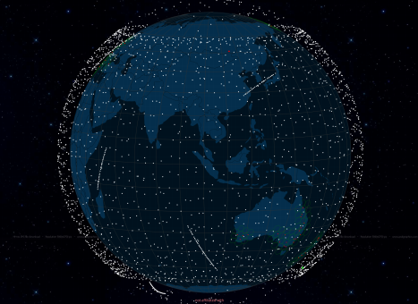
Figure 1: Map of Starlink satellites as of 2023-04-15 using tracker on satellitemap. space.

SpaceX are not the only operators with megaconstellation plans. For example, by the end of the decade, Amazon’s Kuiper constellation plans 3236 satellites in orbit, and OneWeb, 7088 satellites. The deployment of megaconstellations is giving rise to serious concerns about space pollution. At the extreme end of concerns is the worry about triggering Kessler’s syndrome.2 This is a scenario proposed by NASA scientist Donald Kessler in 1978 in which there are so many objects (satellites and debris) in an orbit that collisions between objects cause a cascade leading to an exponential rise in probablity of further collisions. The result would be a debris field that limits further access to space. More moderate concerns about megaconstellatinos have been penned in a letter 3 from

NASA to the US Federal Communications Commission.  Those concerns include:  increase in

potential collisions in low Earth orbit; interference with NASA’s launches; and interference with observation and scientific activities. To counter these concerns, modern satellites can be adjusted in their orbits. Operators monitor for collisions and adjust a satellite’s orbital path with a thrust manoeuvre if required. A long-term Kessler syndrome is unlikely in the orbits where Starlink operates; there is still enough atmospheric drag to bring these satellites out of orbit on the scale of 5– 10 years. These satellites will burn up upon re-entry into the thick Earth atmosphere.

In this assignment, we will not attempt to settle the debate about space pollution due to megaconstellations. We will, however, write computer programs to interact and interrogate a database of known satellites.  In this way, we can at least provide hard evidence to questions about the congestion of satellites in orbit about Earth. For example, it is one thing to be alarmed by the sheer number of satellites in a megaconstellation. However, we should also ask: how much mass does that represent in orbit? We will make use of a database made available by the Union of Concerned Scientists at: https://www.ucsusa.org/resources/satellite-database.  The latest database available is from May 1, 2022. It is compiled from openly-available documents so the data is not entirely complete but it provides a fairly accurate description of what artificial satellites are presently orbiting Earth.

Satellites and basic orbital mechanics

Figure 2(a) shows some satellites in orbit about Earth. The satellites orbiting the Earth are in elliptical orbits (and a circular orbit is a special case of an ellipse). For this reason, the geometry of an ellipse is very useful for computing information about satellite orbits such as the time taken to complete the orbit and the speed of the satellite at points along its orbit. The basic geometry of an ellipse is shown in Figure 2(b). An ellipse is characterised by the lengths of its major and minor axes and its focus points. In an orbital mechanics sense, the satellite only orbits one of the focus points; the Earth is the focal point. We will need to compute some basic orbital parameters in this assignment. The images in Figure 2 provide a visual reference for our calculations. There are two important points on the orbit and they are given special names: (1) the apogee is the point where the satellite is furthest from Earth; and (2) the perigee is the point where the satellite is closest to Earth. In this assignment, the data about a satellite’s orbit will be given in terms of altitudes at apogee and perigee.

Let’s now look at some properties of actual satellites in orbit above the Earth. The properties include those related to the satellite itself and the orbit it occupies.  Table 1 shows data for a small selection of satellites.  Sky Muster 1 — an NBN satellite — and Starlink-1009 are both communications satellites, but the differences between them show the evolving nature of communications satellites technology.  Sky Muster 1 is an example of a single large piece of infrastructure (6440 kg) that sits in geosynchronous orbit so that it permanently services a portion of the Earth (ie.  Australia).  By contrast, Starlink-1009 has a mass of 227 kg and occupies a low Earth orbit.  It moves around the Earth in about 1.5 hours but is part of a much larger constellation, and collectively the constellation can service all regions of the Earth’s surface.

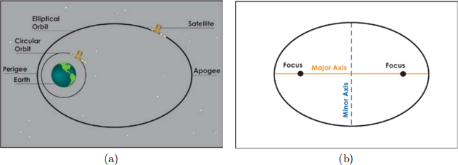
Figure 2: Elliptical orbits.  (a) depiction of satellites in various orbits about Earth; (b) geometry of an ellipse. Source:  UCS Satellite Database User’s Manual [2].

Table 1: Selected satellite data. Apogee and perigee data are altitudes above Earth.

Task 1

Begin your solution in the supplied file a2 .py.

Write a function compute_eccentricity that accepts as parameters the altitude at apogee and the altitude at perigee of a satellite, and the radius of the Earth. The function should return the eccentricity for that orbit. The info box below explains what eccentricity is.

Orbital mechanics – note 1

Eccentricity, e, is the measure of how elliptical an orbit is. Values of eccentricity close to 0.0 are nearly circular, and values near 1.0 are highly elliptical. A circular orbit is a special case of an ellipse and has eccentricity equal to zero. The formula for computing eccentricity based on the altitudes at apogee (ha) and perigee (hp) is:

e = ha − hp

where RE  is the radius of the Earth in kilometres. You can take RE  = 6370 km.

An example console session shows this function in use to compute the eccentricities of Sky Muster 1 and Spektr-R (see Table 1 for relevant orbit data).

>>>  R_E  =  6370

>>>  h_a_sm  =  35777;  h_p_sm  =  35744

>>>  compute_eccentricity(h_a_sm,  h_p_sm,  R_E)

0.0003916402606187916

>>>  h_a_spektr  =  330000;  h_p_spektr  =  1000

>>>  compute_eccentricity(h_a_spektr,  h_p_spektr,  R_E)

0.9571187525455286

Task 2

Orbital mechanics – note 2

The period of an orbit is the time taken for the satellite to travel its orbital path back to a starting point. The period, T , given in units of seconds can be computed using the equation:

where a is the semi-major axis of the orbit and µ is the gravitational parameter.  For Earth, µ = 398600 km3 s −2 .  The semi-major axis, a, can be computed from the apogee and perigee values:

a = (ha+ hp+ 2RE)                                                       (3)

Write a function compute_period that accepts as parameters the altitudes at apogee and perigee for a satellite, the radius of the Earth, and the gravitational parameter for the Earth. The function should return the period of the satellite’s orbit in units of hours. Take note that Equation 2 will give a value of period in seconds, so you will need to do a conversion to hours.

Here is a console session that computes the periods for the Starlink-1009 and Spektr-R satellites using the compute_period function.

>>>  R_E  =  6370; mu  =  398600

>>>  h_a_sl  =  551;  h_p_sl  =  549

>>>  compute_period(h_a_sl,  h_p_sl,  R_E, mu)

1.5913578913826627

>>>  h_a_spektr  =  330000;  h_p_spektr  =  1000

>>>  compute_period(h_a_spektr,  h_p_spektr,  R_E, mu)

196.97396894869757

Task 3

Write a function plot_orbit_path that accepts as parameters the altitudes at apogee and perigee for a satellite, the radius of the Earth, and the number of samples to use in the plot. The function should produce a plot of the orbital path. The equations for determining the (x,y) coordinates for a position in the orbit are described in the next info box.

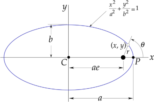
Figure 3:  Cartesian coordinates in relation to ellipse parameters.  Source:  Fig. 2.9 in Curtis (2021) [3]

Orbital mechanics – note 3

Figure 3 shows key geometric parameters of an ellipse. The Cartesian positions, (x,y), can be computed as a function of angle θ using the following: