CS4100/CS5100 Assignment 1
Learning outcomes assessed
The learning outcomes assessed are:• develop, validate, evaluate, and use effectively machine-learning and statistical algorithmsInstructions
• apply methods and techniques such as probabilistic forecasting, logistic regression, and gradient descent
• extract value and insight from data
• implement machine-learning and statistical algorithms in R or MATLAB
In order to submit, copy all your submission files into a directory, e.g., DA, on the server linux and run the script
submitCoursework DA
from the parent directory. Choose CS5100 or CS4100, as appropriate, and Assignment (=exercise) 1 when prompted by the script. You will receive an automatically generated e-mail with a confirmation of your submission. Please keep the e-mail as a submission receipt in case of a dispute; it is your proof of submission. No complaints will be accepted later without a submission receipt. If you have not received a confirmation e-mail, please contact the IT Support team.
You should submit files with the following names:
• GD.R or GD.m should contain the source code for your program (these can be split into files such as GD4.R for task 4, GD6.R for task 6, etc.);
• optionally, other.R or other.m, which are all other auxiliary files with scripts and functions (please avoid submitting unnecessary files such as old versions, back-up copies made by the editor, etc.);
• report.pdf should contain the numerical results and (optionally) discussion.
The files you submit cannot be overwritten by anyone else, and they cannot be read by any other student. You can, however, overwrite your submission as often as you like, by resubmitting, though only the last version submitted will be kept. Submissions after the deadline will be accepted but they will be automatically recorded as late and are subject to College Regulations on late submissions.
Tasks
1. Implement the logistic regression algorithm using Gradient Descent in analogy with neural networks (as described in the lectures, Chapter 4, or [1], Sections 11.3{11.5) for p attributes. The objective function, which your program should minimize, can be either the training MSE
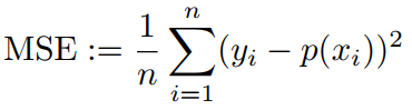
(as described on slide 44 of Chapter 4); the choice is yours. (Be careful mnot to confuse p as the number of attributes and p(x) as the predicted probability of 1.) Your program can be written either in R or in MATLAB. You are not allowed to use any existing implementations of logistic regression or Gradient Descent in R, MATLAB, or any other language, and should code logistic regression from first principles. However, you are allowed to set the number of attributes p to a specific value that allows you to do the following tasks.
2. Use the Auto data set. Create a new variable high that takes values
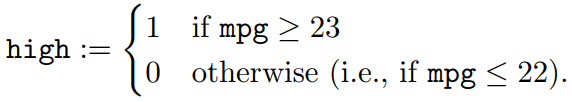
Apply your program to the Auto data set and new variable to predict high given horsepower, weight, year, and origin. (In other words, high is the label and horsepower, weight, year, and origin are the attributes.) Since origin is a qualitative variable, you will have to create appropriate dummy variables. Normalize the attributes, as described in Lab Worksheet 4, Section 5 or Exercise 9 (or Section 4.6.6 of [2]).
3. Split the data set randomly into two equal parts, which will serve as the training set and the test set. Use your birthday (in the format MMDD) as the seed for the pseudorandom number generator. The same training and test sets should be used throughout this assignment.
4. Train your algorithm on the training set using independent random numbers in the range [-0:7; 0:7] as the initial weights. Find the MSE on the test set (it is defined by (1) except that the average should be over the test rather than training set). Try different values of the learning rate η and of the number of training steps (so that your stopping rule is to stop after a given number of steps). Give a small table of test and training MSEs in your report.
5. Optional: Try different stopping rules, such as: stop when the value of the objective function (the training MSE) does not change by more than 1% of its initial value over the last 10 training steps.
6. Run your logistic regression program for a fixed value of η and for a fixed stopping rule (producing reasonable results in your experiments so far) 100 times, for different values of the initial weights (produced as above, as independent random numbers in [-0:7; 0:7]). In each of the 100 cases compute the test MSE and show it in your report as a boxplot.
7. Optional: Redo the experiments in items 4{5 modifying the training procedure as follows. Instead of training logistic regression once using Gradient Descent, train it 4 times using Gradient Descent with different values of the initial weights and then choose the prediction rule with the best training MSE.
Feel free to include in your report anything else that you find interesting.
Marking criteria
To be awarded full marks you need both to submit correct code and to obtain correct results on the given data set. Even if your results are not correct, marks will be awarded for correct or partially correct code (up to a maximum of 70%). Correctly implementing Gradient Descent (Task 1) will give you at least 60%.
Extra marks
It is possible to get extra marks (at most 10%) that will be added to your overall mark (the sum will be truncated to 100% if necessary). Extra marks will be given for doing the optional tasks (5 and 7) and for any interesting observations about the dataset and method (discuss these in your report).
References
[1] Trevor Hastie, Robert Tibshirani, and Jerome Friedman. The Elements of Statistical Learning: Data Mining, Inference, and Prediction. Springer, New York, second edition, 2009.[2] Gareth James, Daniela Witten, Trevor Hastie, and Robert Tibshirani. An Introduction to Statistical Learning with Applications in R. Springer, New York, 2013.
A Details of the algorithm
Please consult this appendix only after you try to derive the algorithm yourself. You should just emulate the derivation on slides 82{88 of Chapter 4 (your task is now easier than that in Chapter 4). I will only give a derivation for the MSE objective function.
The training set is (x1; y1); : : : ; (xn; yn), and we need to estimate the weights β0 and β := (β1; : : : ; βp)0. The training set MSE is
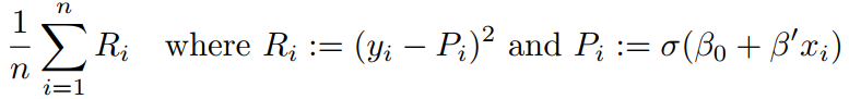
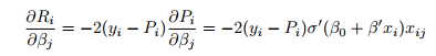
(where j = 0 is allowed; σ0 is the derivative of σ, and in all other cases the prime means transposition). Let us denote
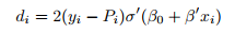
(the coefficient in the partial derivative in front of xij, ignoring the minus sign; it does not depend on j). The overall gradient of the training MSE is given by
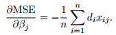
The Gradient Descent algorithm becomes: Start from random weights βj, j = 0; 1; : : : ; p. For a number of epochs (=training steps), do the following:
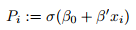
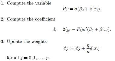
1. \Forward pass": Compute the variable
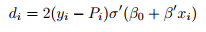
2. \Backward pass": Compute the coefficient
3. Update the weights
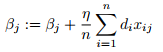
Remember that xij is the jth attribute of the ith training observation (and that xi0 is interpreted as 1).
B An alternative algorithm
It is very easy to make a mistake and implement the following modification of the algorithm described in Appendix A instead of the algorithm itself:
The algorithm Start from random weights βj. Repeat the following for a number of epochs. For each training observation (i = 1; : : : ; n) do the following.
This modification gives reasonable results, is even easier to implement than the version in Appendix A, and you will get full credit for it.
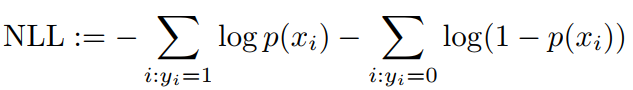
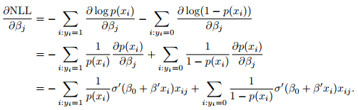
C If you decide to use NLL
If you prefer to use NLL instead of MSE, the gradient is given by:
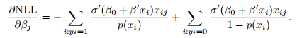
This is the derivation (please check it):
2019-11-07
implement machine-learning and statistical algorithms in R or MATLAB