Instructions:

Assignment:

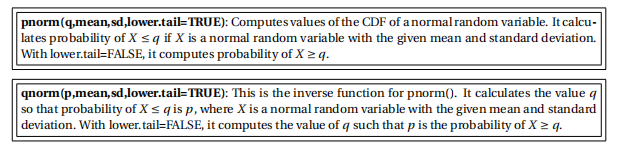
1. Compute each of the following directly . Use pnorm() and qnorm(), or a normal distribution table or calculator, as required.

(a) Suppose that the body temperature of healthy humans is approximately normally distributed with a mean of 98.6 degrees and a standard deviation of 0.8 degrees.

• If 130 healthy people are selected at random, what is the probability that the average temperature for these people is 98.25 degrees or lower?

• Would you consider an average temperature of 98.25 to be an unlikely occurrence, given that the true average temperature of healthy people is 98.6 degrees? Explain.

(b) A balanced coin is flipped 400 times. determine the number x such that the probability that the number of heads is between 200 − x and 200+ x is approximately 0.80.
(c) A surveyor is measuring the height of a cliff known to be about 1000 feet. He assumes his instrument is properly calibrated and that his measurement errors are independent and normally distributed, with mean µ = 0 and variance σ 2 = 10. He plans to take n measurements and form the average.

i. Estimate how large n should be if he wants to be 95% sure that his average falls within 1 foot of the true value?

ii. If µ = 0 is still true, what value should σ 2 have if he wants to make only 10 measurements to be 95% sure that the average of those 10 measurements falls within 1 foot of the true value?

2. Next, download the two data files and open the provided R script. It defines three sets of values:

• example - to demonstrate the code.

• quiz - quiz scores (out of 10) for students.

• lions - weights in pounds for lions at a zoo.

(a) Remember that the Central Limit Theorem can only be used for sufficiently large sets of data taken from an approximately normal distribution. The two plotting techniques used here help to determine if the distribution is approximately normal.
(b) Look at the list of example data, then run the code. Experiment with changing the kernel bandwidth to see how the kernel density function graph changes.
(c) Modify the provided code, adjusting the data used and experiment with the kernel bandwidth.
(d) Visualize the kernel density and quantile -quantile plots for the students’ quiz scores and for the lions ’ weights. Consider these plots together with the sizes of each data set to determine if the central limit theorem is appropriate for that data.
(e) For one of the data fifiles, the conditions to use the central limit theorem aren’ t met. State which. Note any observations you can about that data set that could explain why this is.
(f ) For one of the data fifiles, the conditions to use the central limit theorem are met. For that data, use the estimators µ ≈ x ¯ and σ ≈ sn and the central limit theorem to estimate a number q such that a sample mean X ¯ n for samples of this size has a 95% probability of being below that number. (Your q is called the 95th percentile for this distribution) .