Homework 04: Project
Hello, dear friend, you can consult us at any time if you have any questions, add WeChat: daixieit
Homework 04: Project (20 points)
March 2, 2023
The purpose of this project is to Calculate Market Risk Value at Risk (VaR) and Expected Short Fall (ES) of a portfolio of Zero Coupon Bonds with different maturities. We will do this in various steps.
Note: Submit your code with the answers. (BTW. My code is in Python, but you can use R)
1 Preparing the yield curves (0 points)
The “US treasury.csv”file contains the time-series of annual yield term structure yt , for t =30 days, 90 days, ..., 10950 days (real = 30years). These yields correspond to the discount rate (risk free) one should use to price any instrument on a given time. For example,
a) Assume today is 2007/01/02 and you buy a bond with maturity date 1 year from that date. Hence, the price of a 1yr maturing bond is
B(1yr) = 100e−y365 (365/365) = 100e−0 .0504 = 95.08
since the rate on that date was 5.04% per annum (see Figure 1).
b) Similarly, now assume today is 2022/07/25 (that is, 15+ yrs later) of a 1yr maturing bond is B(1yr) = 100e−y365 (365/365) = 100 * e −0 .030743 = 96.97
since the rate on that date was 3.0743% per annum (see Figure 1).
In this part of the exercise you will prepare the raw data to be useful.
1. If necessary give format to dates dates (If you use python the dates should be transformed into datetime format, e.g., use the pandas.to datetime())
2. Remove dates with missing data: make sure the raws are complete and if not, remove the entire row. The dataframe should look similar to the one on Figure 1.
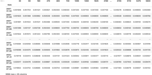
Figure 1: Formatted raw data
Figure 2 illustrates the sample path of yield curves through time. As you can see the nodes are highly correlated, we will discuss this later.
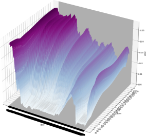
Figure 2: 3D Figure of Yield Curves
2 Principal Components Analysis for yield curves (4 points)
As you can see from Figure 2 the interest rate curves are highly correlated. In fact, some of the correlations will be close to perfect correlation. This means that doing a variable reduction would be useful.
Proceed as follows:
a) Obtain the first differences for each node yti . That is, Xt = Yti − Yti − 1 , where Y is the yields’s matrix (N × M) with N is the length of the time-series, M the number of nodes (e.g., 30days, 90days, ...), see Figure 1. Hint. Make sure you remove rows with “n/a”.
b) Obtain the first 3 principal components (vectors) PCi , i = 1, 2, 3. The PC’s should looks similar to Figure 3 (recall that −PC are also principal components, rotated)
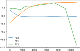
Figure 3: PC’s: PC0 (almost)-parallel shift, PC1 slope, PC2 curvature.
c) Obtain the time series Zi , i = 1, 2, 3 of the principal components as Zt(i) = Xt PCi (matrix multiplication: (N × M) × (M × 3)).
Answer the following:
1. What percentage of variation is explained by each of the 3 PC’s and also cumulatively (PC0,PC0 + PC1,PC0 + PC1 + PC2).
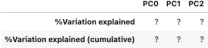
Figure 4: % of Variation of PC’s
2. Plot the time series of PC’s. Recall that X are differences, to see the trajectories of PC’s we need to do the cumulative sum of PC’s time series. That is, plot both graphs.
3. What is the mean, median, standard deviation, skewness and excess kurtosis of the PC’s? Are the PC’s normally distributed? Do you see clusters in the PC’s time-series?
4. What is the correlation of the PC’s time-series?
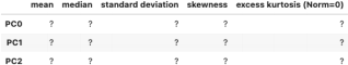
Figure 5: PC’s descriptive statistics
3 The Standard (or Gaussian) Ornstein Uhlenbeck Model (4 points)
3.1 Model description
Consider the stochastic process (Xt )t≥0 described by the SDE,
dXt = κ(θ − Xt )dt + σdBt , Xt ∈ R, t > 0, X0 = x
![]() where κ > 0 is the mean reverting rate, θ ∈ R is the long-run mean, σ > 0 is the volatility and (Bt )t≥0 is a Brownian motion. The solution to this SDE is given by
where κ > 0 is the mean reverting rate, θ ∈ R is the long-run mean, σ > 0 is the volatility and (Bt )t≥0 is a Brownian motion. The solution to this SDE is given by
Xt = θ (1 − e −κt)+ xe−κt + σ\0 t e −κ(t−s)dBs , t ≥ 0 (3.1)
![]()
![]() to obtain
to obtain
![]() E[Xt |X0 = x] = xe−κt + θ (1 − e −κt)
E[Xt |X0 = x] = xe−κt + θ (1 − e −κt)
and
Cov (Xt ,Xs |X0 = x) = E[(Xt − E[Xt]) (Xs − E[Xs])] = ![]() (e −κ|t−s| − e −κ(t+s))
(e −κ|t−s| − e −κ(t+s))
which is independent of X0 = x. Hence,
![]() Var(Xt |X0 = x) =
Var(Xt |X0 = x) = ![]() (1 − e −2κt) .
(1 − e −2κt) .
3.2 Parameter estimation
The Ornstein Uhlenbeck process is closely related to the Autorregressive AR(1) process. In fact, consider Xt to be observed at discrete times X = (Xt0 ,Xt1 , . . . ,XtN ) = (x1 ,x2 , ··· ,xN ) where the time interval between
Xti = xi and Xti − 1 = xi−1 is ∆t = ti − ti−1 . Thus we can discretize the OU process given in Eq. (3.1) as
xi = θ(1 − e −κ∆t) + e −κ∆txi−1 + ![]() (1 − e −2κ∆t)z, z ∼ N(0, 1) (3.4) where we used It´o isometry, E [ (l0(t) Yu dBu )2] = E [l0(t) Yu(2)du] for Yt adapted to Ft = σ({Bu : u ≤ t}).
(1 − e −2κ∆t)z, z ∼ N(0, 1) (3.4) where we used It´o isometry, E [ (l0(t) Yu dBu )2] = E [l0(t) Yu(2)du] for Yt adapted to Ft = σ({Bu : u ≤ t}).
Hence, Eq. (3.4) can be written as a linear equation,
xi = a + bxi−1 + ϵ
Using Ordinary Least Squares we can find the parameters a,b and the residuals ϵ . From these we obtain the OU parameters,
![]() ln(b)
ln(b)
∆t
a
![]() 1 − b
1 − b
σ = Std(ϵ) −2ln(b)
√∆t (1 − b2 )
Next, consider the case of multivariate OU process, that is,
Xt(j) = θj (1 − e −κj t )+ xj e −κj t + σj \0 t e −κj (t−s)dB s(j), t ≥ 0, X0(j) = xj
Such that,
Corr(Bt(k),Bt(j)) = ρk,j
It can be easily shown that using the set of residuals ϵ obtained for each processes, ρk,j = Corr(ϵk ,ϵj )
3.3 Questions
Assume that each yield rate Yti follows an OU process as in Eq. (3.1). In what follows assume ∆t = ![]() .
.
1. Estimate the OU parameters θ,κ,σ for each node (30, 90, . . . ). In particular, what are the parameters for nodes: 90,1460, 5110 and 7300?
2. Estimate the correlation of the OU parameters ρij for each node. In particular, what is the correlation matrix for nodes: 30,90,180,7300,9125 and 10950?
4 Monte Carlo Simulation (4 points)
From Eqs. (3.1), (3.2) and (3.3) we can see that the OU process is normally distributed N(![]() t ,
t , ![]() t(2)) with the mean and standard deviation depending on time and the initial state,
t(2)) with the mean and standard deviation depending on time and the initial state,
Thus to simulate a sample path over a grid of time steps T = {t0 ,t1 , . . . ,tN } we do it sequentially considering the previous state Xti to obtain the next state Xti+1 by drawing a random variable from a normal distribution using (4.5) and (4.6).
Pseudo Code
1. Generate the time-grid T = {t0 ,t1 , . . . ,tN }
2. Set x[0] = Xt0
3. For i ∈ {1, 2, ...,N}:
(a) Obtain ![]() t and
t and ![]() t using x[i − 1] and (t − s) = ti − ti−1
t using x[i − 1] and (t − s) = ti − ti−1
(b) Draw a r.v. z from N(![]() t ,
t , ![]() t(2))
t(2))
(c) Set x[i] = z
The previous code can be easily extended to the multivariate case since the multivariate OU process (Xt(1),Xt(2) , . . . ,Xt(n)) has a multivariate normal distribution N(![]() t ,
t , ![]() t ) where
t ) where ![]() t = (
t = (![]() t(1) , . . . ,
t(1) , . . . , ![]() t(n)) and
t(n)) and ![]() t = Dρt D where D = Diag(σ1 , . . . ,σn ) (diagonal matrix of the instantaneous volatilities σi’s), and where ρt (time- dependent) is given by the matrix whose elements are,
t = Dρt D where D = Diag(σ1 , . . . ,σn ) (diagonal matrix of the instantaneous volatilities σi’s), and where ρt (time- dependent) is given by the matrix whose elements are,
![]() ( 1 − e −(κi +κj )(t−s))
( 1 − e −(κi +κj )(t−s))
Here ρi,j is the instatanenous correlation of Brownian motions.
4.1 Questions
1. Draw a single three-year (3 × 365 days) sample path of daily realizations for all nodes. Use the values of 2022/07/25 as your initial vector. Then draw a 3-D plot with your sample. Below is an example of a 5 year simulation
5 Value at Risk and Expected Shortfall (8 points)
Assume that today is 2022/07/25 and you hold two bonds (two long positions):
a) A bond maturing 730 days (2 year) from now and pays $100 at maturity.
b) A bond maturing 1095 days (3 years) from now and also pays $100 at maturity.
5.1 Questions
1. What is the value of the bonds and of your portfolio today (2022/07/25)?
2. Assuming that you are interested in 1 year time-horizon for your analysis, i.e., 365 days in the future. If the yield rates remain constant for one year, what is the value of the bonds and of your portfolio in
1 year from today? and what would be the value of that portfolio today (today’s dollars)?

Figure 6: 3D Figure of MC simulation of Yield Curves
Hint: One year from today the bonds have 365 days less to maturity, and since the time-horizon is too long, you need to discount that value to today’s dollar.
3. Compute 100,000 Monte Carlo simulations to answer the following questions.
Hint: You don’t need to simulate all nodes, and you don’t need to simulate daily increments. Recall also, that you need to discount the values to today’s dollars since the time-horizon is long.
(a) What is the 1 year VaR at 99% confidence (express it in terms of losses in relation to today’s
value, i.e. first question)?
(b) What is the 1 year ES at 99% confidence (express it in terms of losses in relation to today’s value,
i.e. first question)?
2023-03-16