CHE1148H - Data Process Analytics Programming assignment #2
Hello, dear friend, you can consult us at any time if you have any questions, add WeChat: daixieit
Programming assignment #2
Course: CHE1148H - Data Process Analytics
Some notes
If you took CHE1147, this looks familiar; it is one of the assignments on feature engineering. Regardless, the situation is that our company is growing from a startup to a bigger organi- zation and we now want to migrate the Python code we developed and ran on our laptops with small datasets to a big data/cloud architecture in Databricks.
You’ve been hired to do this migration. This is actually a very realistic scenario and possi- bly your work for a whole year: migrate features and models. The documentation of the old Python code below is all you have. You have to find out how to perform the transformations in PySpark. Some steps will be identical to plain Python, some will be different, some will not be needed at all.
1 Feature engineering
Here, you are going to create features from a very simple dataset: retail transaction data from Kaggle. The dataset provides the customer ID, date of the transaction and transaction amount as shown in the table below. Although this may look like a very simple dataset, you will build a wide range of features0. The features will then be used as inputs in several models in upcoming assignments, in which you will try to predict the client’s response to a promotion campaign.
1.1 Import the data and create the anchor date columns
In order to create features, you need to create some anchor dates. The most typical for transaction data is the end of the month and the year.
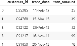
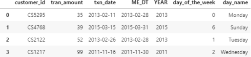
1. Import the dataset as txn1 and identify the number of rows2.
2. The date-format in column ’trans date’ is not standard. Create a new column ’txn date’ from ’trans date’ with pd.to datetime and drop the column ’trans date’ .
3. Identify the min() and max() of column ’txn date’ .
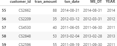
4. Create the column ’ME DT’: the last day of the month in the ’trans date’ column. DateOffset objects is a simple way to do this in pandas.
5. Create the column ’YEAR’: the year in the ’trans date’ column. DatetimeIndex with attribute .year will help you do so.
The table output should look like the snapshot below. Make sure that the column ’ME DT’ works as expected. E.g. for the first line ’trans date’: 2018-08-31 is converted to 2018-08-31. A common mistake in implementing the DateOffset transformation is to convert 2018-08-31 to 2018-09-30 (a date that falls on the last day of a month is converted to the last day of the next month!!!).
1.2 Create features that capture annual spending
Here the approach is to capture the client’s annual spending. The rationale behind this approach is that the clients spend is not very frequent to capture in a monthly aggregation.
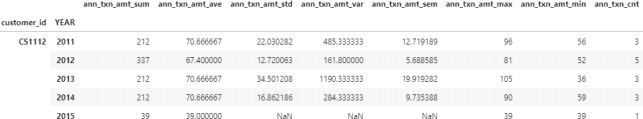
1. Using groupby and NamedAgg create clnt annual aggregations, the annual aggre- gations dataframe: with sum, mean, std, var, sem, max, min, count as the aggregation functions. A snapshot of the output table is shown below. Notice that the output is a typical MultiIndex pandas dataframe.
2. Plot the histogram of the sum and count.
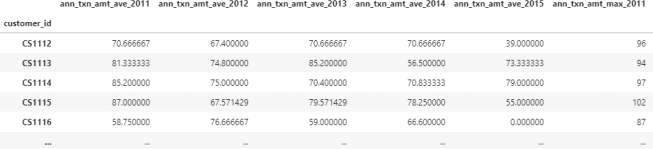
3. Reset the index and reshape the table with the pivot table function to create the clnt annual aggregations pivot table shown below with 40 columns (why 40?).
You should expect columns with NaN values. Impute the NaN entries when you perform the pivot table function and explain your choice of values.
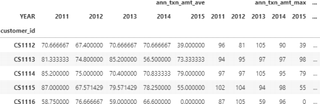
4. The pivoted object you created is a MultiIndex object with hierarchical indexes. You can see the first level (i.e. 0) in the snapshot above with names ’ann txn amt ave’, ’ann txn amt max’ (and more as indicated by the ...) and the second level (i.e. 1) with names ’2011’, ’2012’, etc. You can confirm the multiple levels of the columns with the following two expressions.
What are your observations regarding the number of levels and the column names?
|
c l n t _ a n n u a l _ a g g r e g a t i o n s _ p i v o t . columns
|
5. Finally, you want to save the dataframe clnt annual aggregations pivot as an .xlsx file for future use in the machine learning assignment. To do so, you want to remove the two levels in columns and create a single level with column names: ’ann txn amt ave 2011’, ’ann txn amt ave 2012’, etc. To do so, use the code snippet below prior to saving the dataframe as an Excel file.
|
level _ 1 = c l n t _ a n n u a l _ a g g r e g a t i o n s _ p i v o t . columns . g e t _ l e v e l _ v a lu es ( 1 ) . astype ( str ) c l n t _ a n n u a l _ a g g r e g a t i o n s _ p i v o t . columns = level _ 0 + ’_ ’ + level _ 1 |
Describe what each line of code in the box does and save the output dataframe as an Excel file annual features.xlsx. A snapshot of the desired final output is shown below.
6. What are the possible disadvantages in capturing client transaction behavior with the annual features described in this section (if any)?
1.3 Create monthly aggregations
Here, you want to explore the monthly sum of amounts and count of clients transactions.
1. Create the dataframe that captures the monthly sum and count of transactions per client (name it clnt monthly aggregations). Use the groupby function with the Named Aggregation feature which was introduced in pandas version 0.25.0. Make sure that you name the columns as shown in the figure sample on the right.
2. Create a histogram of both columns you cre- ated. What are your observations? What are the most common and maximum values for each column? How do they compare with the ones in section 1.2?
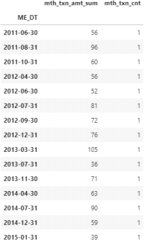
The output dataframe should look like the snap- shot shown on the right for client with ID CS1112 (confirm this with slicing your output dataframe).
Most clients in this dataset shop a few times a year. For example, the client with ’customer id’ CS1112 shown here made purchases in 15 out of 47 months of data in the txn table. The information in this dataset is ”irregular”; some clients may have an entry for a month, while others do not have an entry (e.g. when they don’t shop for this particular month).
1.4 Create the base table for the rolling window features
In order to create the rolling window features (more on this in the next section), you need to create a base table with all possible combinations of ’customer id’ and ’ME DT’ . For example, customer CS1112 should have 47 entries, one for each month, in which 15 will have the value of transaction amount and the rest 32 will have zero value for transaction amount. This will essentially help you convert the ”irregular” clnt monthly aggregations table into a ”regular” one.
1. Create the numpy array of the unique elements in columns ’customer id’ and ’ME DT’ of the txn table you created in section 1.1. Confirm that you have 6,889 unique clients and 47 unique month-end-dates.
2. Use itertools.product to generate all the possible combinations of ’customer id’ and ’ME DT’ . Itertools is a Python module that iterates over data in a computation- ally efficient way. You can perform the same task with a for-loop, but the execution may be inefficient. For a brief overview of the Itertools module see here. If you named the numpy arrays with the unique elements: clnt no and me dt, then the code below will create an itertools.product object (you can confirm this by running: type(base table)).
|
base _ table = product ( clnt _no , me _ dt ) |
3. Next, you want to convert the itertools.product object base table into a pandas ob- ject called base table pd. To do so, use pd.DataFrame.from records and name the columns ’CLNT NO’ and ’ME DT’ .
4. Finally, you want to validate that you created the table you originally wanted. There are two checks you want to perform:
❼ Filter client CS1112 and confirm that the dates fall between the min and max
month-dates you identified in section 1.1. Also, confirm that the snapshot of client CS1112 has 47 rows, one for each month in the dataset.
❼ Confirm that the base table pd has 323,783 rows, which is the expected value
of combinations for 6,889 unique clients and 47 unique month-end dates.
1.5 Create the monthly rolling window features
With the base table pd as a starting point you can convert the irregular transaction data into the typical time series data; data captured at equal intervals. Feature engineering of time series data gives you the potential to build very powerful predictive models.
1. Left-jointhe base table pd with the clnt monthly aggregations table from section 1.3 on [CLNT NO, ME DT] to create the table base clnt mth. Comment on the following questions in Markdown:
❼ Why do some rows have NaN values?
❼ What values will you choose to impute NaN values in the sum and count columns?
Perform the imputation you suggest.
❼ Confirm that the number of rows is what you expect. What is the value?
❼ How are tables base clnt mth and clnt monthly aggregations different? Com-
ment on the number of rows and the content of each table.
2. For the next step, the calculation of the rolling window features, you need to sort the data first by ’CLNT NO’ and then by ’ME DT’ in ascending order. This is necessary to create the order for rolling windows, e.g. 2011-05-31, 2011-06-30, etc.
3. The idea behind rolling window features is captured in the image below. You calculate some statistical properties (e.g. average) based on a window that is sliding. In the image below, the window is 7 which means that the last 7 points are used at every row to calculate the statistical property.
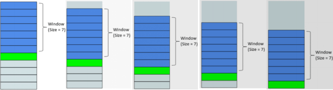
Here, you have to calculate separately the 3, 6 and 12-month rolling window features (tables: rolling features 3M, rolling features 6M, rolling features 12M) for every client that calculates the aggregations ’sum’, mean’ and ’max’ for both columns ’mth txn amt sum’ and ’mth txn cnt’ . The steps to achieve this with base clnt mth as the starting dataframe are:
❼ groupby the client number
❼ select the two columns you want to aggregate
❼ use the rolling function with the appropriate windows
❼ aggregate with ’sum’, mean’ and ’max’
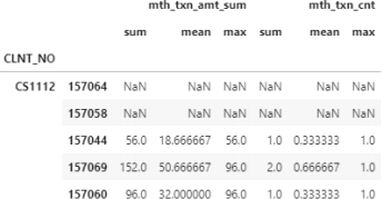
The output of the 3-month rolling window dataframe is shown below. Also, answer the following questions in the .ipynb notebook as Markdown comments.
❼ How many rows appear with NaN values at the beginning of each client for 3, 6
and 12-month windows, respectively? Why do they appear?
❼ How many levels do the index and columns have? Are these MultiIndex dataframes?
❼ Rename the columns as following: ’amt sum 3M’, ’amt mean 3M’, ’amt max 3M’,
’txn cnt sum 3M’, ’txn cnt mean 3M’, ’txn cnt max 3M’ and follow the same nam- ing convention for 6M and 12M.
4. Merge the 4 tables: base clnt mth, rolling features 3M, rolling features 6M, rolling features 12M in the output all rolling features. It is recommended to drop the level:0 of the rolling features MultiIndex table and join with base clnt mth on the indexes.
Make sure you understand why joining on the indexes preserves the CLNT NO and ME DT for each index.
5. Confirm that your final output all rolling features has 323,783 rows and 22 columns and save it as mth rolling features.xlsx.
1.6 Date-related features: date of the week
In this section, you will create the date-related features that capture information about the day of the week the transactions were performed.
1. The DatetimeIndex object you used earlier allows you to extract many components of a DateTime object. Here, you want to use the attributes dt.dayofweek and/or dt.day name() to extract the day of the week from column ’txn date’ of the txn table (with Monday=0, Sunday=6). The expected output below shows both columns.
2. Create the bar plot that shows the count of transactions per day of the week.
3. Following the same logic as in section 1.2, generate the features that capture the count of transactions per client, year and day of the week. The intermediate MultiIndex dataframe (with nlevels=3) and the final pivoted output with a single index are shown in the snapshots below.
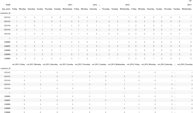
4. Confirm that your output has the same number of rows as the final output in section 1.2 and save it as annual day of week counts pivot.xlsx. How many features/columns did you create in this section?
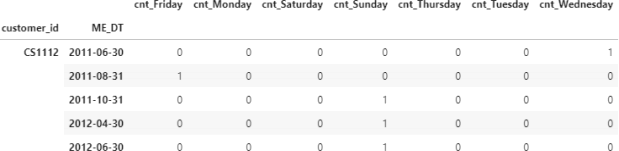
5. Similarly, generate the features that capture the count of transactions per client, month-end-date and day of the week. In contrast with the annual pivot table in the previous step, here you want to create the pivot with [’customer id’, ’ME DT’] as index to obtain the following output dataframe.
6. Join with base table pd as you did in section 1.5 and impute with your choice of value for NaN. Save the final output as mth day counts.xlxs.
1.7 Date-related features: days since last transaction
In this date-related features set, you want to capture the frequency of the transactions in terms of the days since the last transaction. This set of features applies only to the monthly features.
1. The starting point is again the txn table. Recall that most clients have a single purchase per month, but some clients have multiple purchases in a month. Since you want to calculate the ”days since last transaction”, you want to capture the last transaction in a month for every client.
Use the appropriate groupby to create the table last monthly purchase that cap- tures the last ’txn date’ (aggfunc=max) for every client and month.
2. Join base table pd with last monthly purchase as you did in section 1.5. The snapshot below shows the output of the created object last monthly purchase base for client CS1112 who made her/his first purchase on June 2011, then no purchase on July and made a purchase again on August 2011. What values will you use to impute the NaT values here? NaT stands for ”Not a Timestamp” .
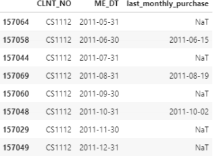
3. To answer the imputation problem, we have to think what value should we use for say July 2011 for ’last monthly purchase’? The answer is that in July the value for the last monthly purchase is the previous line value: 2011-06-15. In other words, for every client we want to forward-fill the NaT values.
While pandas fillna() method has a method to forward-fill, here we want to use the apply and a lambda function with the forward-fill function ffill(), with the follow- ing expression: .apply(lambda x: x .ffill()) applied on object last monthly - purchase base grouped by CLNT NO. Below, I am showing a snapshot for lines [92:98] that confirm the transition between clients CS1113 and CS1114.
You can also recreate the forward-fill with the fillna() method, however there is a disadvantage and a reason the .apply() method is preferred here.
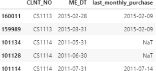
The forward-fill on the grouped by CLNT NO object is expected to leave NaT values for the first months of every client until they purchase something. The above snapshot confirms that for client CS1114.
4. Subtract the two date columns and convert the output to .dt.days to calculate the column ’days since last txn’ as shown in the following snapshot.

5. Plot a histogram of the ’days since last txn’ . Based on the values you observe in the histogram, impute the remaining NaN values (i.e. for the initial months before a client makes a purchase). Save the columns [’CLNT NO’, ’ME DT’, ’days since last txn’] as days since last txn.xlsx.
2023-03-14