闪电代写 -代写CS作业_CS代写_Finance代写_Economic代写_Statistics代写_代码代做_IT代写_加急帮助

Hello, dear friend, you can consult us at any time if you have any questions, add WeChat: daixieit

AM 147: Computational Methods and Applications: Winter 2023

Homework #8

Due: March 08, 2023

Problem 1

Estimate true signal from measured noisy signal (50 points)

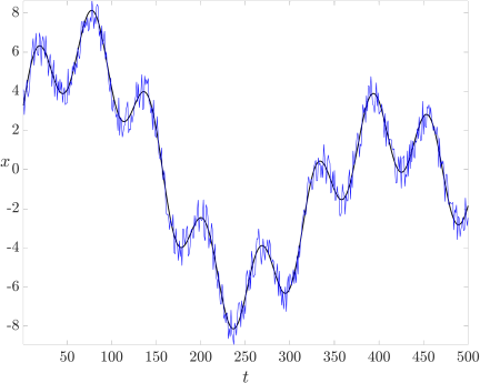
Download the starter code W23HW8.m from CANVAS Files section folder“HW Problems and Solutions”to your computer, and rename it as YourlastnameYourfirstnameHW8.m. The starter code plots a true signal x(t) (in solid black) that is NOT known. Only the noise corrupted signal xnoisy(t) (in solid blue), as shown in the plot above, is available as a sensor measurement. As data scientist, your job is to recover an estimate (t) of the true signal from the noisy measured signal xnoisy(t). We think of t as time; the noisy signal was measured at 500 different time instances.

This problem can be formulated as

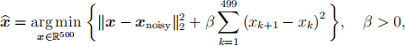(1)

where xk denotes the kth entry of the vector x.

We can interpret the above optimization problem as follows. Since we want the recovered signal to be close to the measured signal xnoisy , it makes sense to minimize x − xnoisy 2(2) . This justiﬁes the ﬁrst summand in the objective. We also want the estimated signal to be “smooth” in the sense it should not change too rapidly between consecutive times. To mathematically capture this, the second summand penalizes rapid changes in the signal between consecutive times. The known parameter β > 0 is ﬁxed. Therefore, the ﬁrst summand in the objective represents data ﬁdelity; the second summand in the objective promotes regularization/smooth- ness. Large β implies smoother but larger mismatch with the measured signal. Similarly, small β implies better match with the measured but more “spiky” signal. For numerical solution, you need to rewrite problem (1) in the standard least squares form

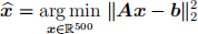
for some appropriately deﬁned tall matrix A and vector b.

Your job is to complete the starter code by typing in some lines between lines 25 and 30. Then uncomment lines 32–43 and complete line 37 within the for loop. The completed code should make a plot of the estimated signals for β = 1, 10, 100 together with the blue and black curves shown above, all in the same ﬁgure.

In the zip ﬁle containing your MATLAB code, please also include a ﬁle named YourlastnameY ourfirstnameHW8.pdf that clearly shows your hand calculations in deriving the tall matrix A and vector b appearing in the standard least squares form.