CSC 263 H1 Problem Set # 4 Winter 2023
Hello, dear friend, you can consult us at any time if you have any questions, add WeChat: daixieit
CSC263H1
Problem Set #4
Winter 2023
General Instructions
• Worth: 2%. Please read the completion requirements carefully (see the last point below).
• Due: By 21:00 on Friday 10 March 2023, on MarkUs. Submissions will be accepted up to one week late with a penalty of −10% for each weekday late (penalties begin at 21:00 on Sunday following the due date). Submissions later than one week will receive no credit.
• Problem sets are to be submitted individually. You are free to discuss the problems and their solutions with others, but you must write and submit your own individual answers. See the section on the Syllabus about Academic Integrity for details of exactly what is allowed and what is not.
• Submissions may be typeset or handwritten legibly, but must be made in a single document in an accepted format — documents that cannot be displayed directly on MarkUs will not be marked, even if MarkUs allows you to submit them. We recommend (but do NOT require) the use of LATEX to produce high-quality documents.
• Remember that your submission must meet specific conditions to receive credit. Please read the Syllabus (https://q.utoronto.ca/courses/293389#problem-sets) for full details of how to benefit the most from
this problem set, and how to submit your work.
Problems
Review
“Review” problems can be solved using only knowledge from prerequisite courses. This does not necessarily mean that they are easy, but they require no new knowledge.
(There is no“review”problem on this problem set.)
Practice
“Practice”problems are straightforward applications of the course material. No creativity or insight should be required to solve them.
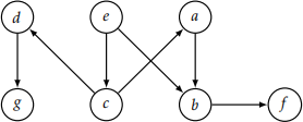
1. For the following graph, write down the set of nodes and edges, as well as the graph’s adjacency matrix and list representations.
2. Consider the following algorithm.
0. FindLast(A, k):
1. i = len(A) − 1
2. while i ≥ 0 and A[i] 才 k:
3. i = i − 1
4. return i
Perform an average-case analysis of FindLast. Define clearly your sample space, probability distribution, random variables, what key operation(s) you are counting, and show your work.
3. Using the steps below, work through an amortized analysis of a stack that in addition to Push and Pop, has a “MultiPop”operation.
0. MultiPop(S, k):
1. while not IsEmpty(S) and k 才 0:
2. Pop(S)
3. k = k − 1
(a) What is the worst-case time complexity of each of the operations Push, Pop and MultiPop on a stack of n items? Assume that IsEmpty is a constant time function.
(b) Calculate a loose upper bound on the worst-case time for n operations by taking the time of the slowest operation (from the previous part) and multiplying by n.
(c) Would it really be possible to have a sequence of n of that operation? If it is possible, would each of the n calls actually take the worst-case time? Either give an example (use a small n) or explain why not.
(d) Using aggregate analysis, argue for a better bound for the total time taken by any sequence of n operations, starting from an initially empty stack.
(e) Then divide by n to obtain the amortized time of a single operation.
Challenge
“Challenge”problems require some insight or creativity to apply the course material in a different way. Challenge- level problems are not necessarily difficult: for example, the first problem below is really more practice-level.
4. Consider the following algorithm. We want to analyze its average-case runtime complexity, counting the number of times we access a list element as the operation of interest. Assume that the subroutine used to implement line 1 is very dumb: even when it encounters a non-even number, it always examines all n numbers (it does not stop early).
0. EvensAreBad(lst):
1. if every number in lst is even:
2. repeat len(lst) times:
3. calculate and print the sum of lst
4. return False
5. else:
6. return True
Be clear about your sample space of inputs, the probability distribution over the sample space, and show your work.
5. Analyze the Increment operation on a decimal counter that starts with all digits at zero. Use the accounting method, with a cost of $1 to represent the real cost of changing a digit. Here is a reminder of the Increment algorithm, where A is an array that stores the digits of the counter.
0. Increment(A):
1. i = 0
2. while i < len(A) and A[i] == 9:
3. A[i] = 0
4. i = i + 1
5. if i < len(A):
6. A[i] = A[i] + 1
6. Conduct an amortized analysis of insertions into a dynamic array where the expansion factor is 1.5 (rounded up). Use the code from the Discover: Dynamic Arrays activity on Quercus. When we calculated the worst-case performance for the original implementation (with an expansion factor of 2), we counted only array accesses. We determined that these only happened on lines 10 and 5. When the underlying array had room for a new element, insert only required one access on line 10. But when the underlying array was full with n elements, inserting one more required 2n accesses on line 5 and then one more on line 10. Now, you must redo the analysis based on changing lines 4 and 7 to multiply the quantity A.allocated by a factor of 1.5 and rounding up (taking the ceiling).
(a) Initially redo the analysis using a charge of $5 for each Insert. Is this enough of a charge? Why or why not?
Show your work.
(b) Find an appropriate charge for each Insert, then state a credit invariant and prove it. Use your invariant to draw an appropriate conclusion for the amortized complexity of each Insert.
Extra
7. If you have to merge two min-heaps H1 and H2 implemented as complete binary trees stored in fixed-sized array, the fastest algorithm is to concatenate the two arrays (place all the values in H1 followed by all the values in H2), then run Build-Min-Heap. This takes linear time (as a function of the total number of elements).
If this is a common operation, we would like to be able to do better. One implementation that achieves this is the binomial heap — careful: binomial heaps are NOT the same thing as binary heaps! Read Problem 19-2 (binomial trees and binomial heaps) in CLRS (p. 527).
Next, answer parts (a), (b), and (c) of problem 19-2 in CLRS.
Finally, show that the amortized complexity of Insert is constant for binomial heaps.
2023-03-08